Poisson Distribution Table
Poisson distribution table for P(X = k) and cumulative P(X ≤ k), λ 0.1 to 20, plus a calculator for λ up to 10,000 and a probability chart. Print or download.
Poisson probability calculator
Plot these probabilities as a bar chart
P(X = 3)
0.2138
P(X ≤ 3)
0.7576
P(X ≥ 3)
0.4562
P(X < 3)
0.5438
P(X > 3)
0.2424
Mean λ
2.5
Variance λ
2.5
Standard deviation
1.58114
Chart style
Poisson probability tables, λ = 0.1 to 20
Choose a block of λ, then read down to k and across to λ. The first tab gives the probability of exactly k events, the second the probability of k or fewer. Click any cell to highlight its row and column.
Mean number of events λ
Export style
Paper for print
| k \ λ | 1.5 | 2.0 | 2.5 | 3.0 | 3.5 | 4.0 | 4.5 | 5.0 |
|---|---|---|---|---|---|---|---|---|
| 0 | ||||||||
| 1 | ||||||||
| 2 | ||||||||
| 3 | ||||||||
| 4 | ||||||||
| 5 | ||||||||
| 6 | ||||||||
| 7 | ||||||||
| 8 | ||||||||
| 9 | ||||||||
| 10 | ||||||||
| 11 | ||||||||
| 12 | ||||||||
| 13 | ||||||||
| 14 | ||||||||
| 15 |
0.0000 means the probability is below 0.00005. It is not exactly zero.
Blank cells: each column stops at the first k where P(X ≤ k) is 0.9999 or more, so a blank cell lies below that point and the blank cells together hold less than 0.0001 of probability. For longer tails, or a λ that is not a column, use the calculator, which accepts any λ up to 10,000.
Values are rounded to four decimals. We compared every printed cell (1,394 in all) with SciPy (poisson.pmf and poisson.cdf) and none differs after rounding.
Selected cell
λ = 2.5, P(X = 3) = 0.2138
More digits: 0.2138. Largest k in this column: 10 of 15 in this block.
Free Poisson Distribution Table Charts
Every chart below is drawn from the same code as the tool above. View, download and print them free, no sign-up.
Poisson Distribution Table: P(X = k), λ 1.5 to 5
Exactly-k probabilities for eight values of λ. For λ = 2.5 and k = 3 the entry is 0.2138.
Reference tables
How to read
Distribution
Printable versions
Counting trials with a fixed chance? Use the binomial distribution table. For large λ, look up normal areas in the z table, and draw a probability bar chart with the bar chart maker. Not sure which table to use? See statistics tables.
What a Poisson distribution table shows
- A Poisson distribution table lists probabilities for a count of events in a fixed interval of time or space: customers arriving in an hour, bacterial colonies on a small area of a plate, mutations in a stretch of DNA. The only parameter is λ (lambda), the average number of events per interval.
- The Poisson model fits when events happen one at a time, independently of each other, at a steady average rate, and the number of events in one interval does not change the chance in another. If events cluster, the counts vary more than the model expects and the Poisson is a poor fit. A useful check is that the mean and the variance of a Poisson count are both λ.
- The probability of exactly k events is P(X = k) = e^(−λ) λ^k ÷ k!, with mean λ and variance λ. The rate scales with the interval: 2.5 arrivals per hour is λ = 5 for a two-hour window.
How to read the table in three steps
- Step 1: find the column for your λ. Step 2: go down to the row for k. Step 3: read the cell. In the individual tab, λ = 2.5 and k = 3 gives 0.2138, so the chance of exactly 3 events is 0.2138. In the cumulative tab the same position gives 0.7576, the chance of 3 or fewer. That entry is the sum of the first four individual entries: 0.0821 + 0.2052 + 0.2565 + 0.2138 = 0.7576. The cumulative entry is the exact sum rounded once, so adding rounded entries can occasionally differ in the last digit.
- A 0.0000 in the table is rounded, not exact. Each column also stops at the first k where P(X ≤ k) reaches 0.9999, and the blank cells below it together hold less than 0.0001 of probability. For a longer tail or a λ between the columns, use the calculator, which takes any λ up to 10,000.
At least, more than, fewer than
- The cumulative tab answers “k or fewer”. The other questions are one subtraction away. P(X ≥ k) = 1 − P(X ≤ k − 1). P(X > k) = 1 − P(X ≤ k). P(X < k) = P(X ≤ k − 1). For λ = 2.5, the chance of at least 4 events is 1 − 0.7576 = 0.2424. For a range, P(a ≤ X ≤ b) = P(X ≤ b) − P(X ≤ a − 1). The calculator at the top gives all five single-k probabilities, and the range for a to b, in one go.
Worked examples: arrivals, colonies, mutations
- Arrivals. A help desk gets 2.5 calls per hour on average. The chance of at most 1 call in an hour is 0.2873, and the chance of more than 5 is 0.0420.
- Colonies. A small area of a plate has on average 0.3 colonies. The chance of finding none is 0.7408, the λ = 0.3, k = 0 entry.
- Mutations. If samples carry on average 1.5 mutations in a region, the chance of 3 or more in one sample is 0.1912. For λ = 10 and at least 15 events, P(X ≥ 15) = 0.0835, a tail value the table gives by subtraction and the calculator gives directly.
- Large λ is no problem for the calculator. For λ = 100 and k = 120, P(X ≤ 120) = 0.9773, P(X ≥ 120) = 0.0282, and P(80 ≤ X ≤ 120) = 0.9599.
Poisson approximation to the binomial
- When n is large and p is small, a binomial count is close to Poisson with λ = np. Common rules of thumb ask for n ≥ 20 and p ≤ 0.05, and some books use n ≥ 100 with np ≤ 10. These are guidelines, not guarantees, and the approximation improves as n grows and p shrinks.
- Example: n = 100 and p = 0.03 gives λ = 3. The exact binomial P(X ≤ 2) is 0.4198 and the Poisson value is 0.4232. If you can use the exact binomial table, do; use the Poisson when n is beyond the table or only the rate is known.
Normal approximation when λ is large
- For large λ the Poisson distribution looks like a normal distribution with mean λ and standard deviation √λ. A common rule of thumb asks for λ ≥ 10, and some texts use 20 or more. Add a continuity correction because the Poisson is discrete: P(X ≤ k) is approximately Φ((k + 0.5 − λ) ÷ √λ).
- Example: λ = 36 and P(X ≤ 40). The exact value is 0.7771. The normal approximation with the correction, Φ((40.5 − 36) ÷ 6), gives 0.7734. Without the correction, Φ((40 − 36) ÷ 6) gives 0.7475, which is further off. For a z-score lookup, use the z table.
Reporting a Poisson probability
- State the model, the rate and the interval, then the probability. In APA style, a probability that cannot exceed 1 is written without a leading zero and usually to two or three decimals: “Arrivals per hour were modeled as Poisson with λ = 2.5; the probability of exactly 3 arrivals was P(X = 3) = .214.” Say how λ was estimated, and whether the counts look Poisson, for example by comparing the sample mean and variance.
Frequently Asked Questions
Related Statistics Tools
 Research
Binomial Distribution Table
Binomial distribution table for n = 1 to 20 and 25 with individual P(X = k) and cumulative P(X ≤ k) values, a calculator up to n = 1000, and printable sheets.
 Research
Bar Chart Maker
Create horizontal, grouped, and stacked bar charts for rankings, comparisons, and classroom data visualization.
 Research
AI Histogram Maker
Create professional histograms and frequency distribution charts for statistics, data analysis, and STEM education.
 Research
Bell Curve Generator
Create professional bell curves and normal distribution graphs for statistics, data analysis, and academic papers.
 Research
Z Table
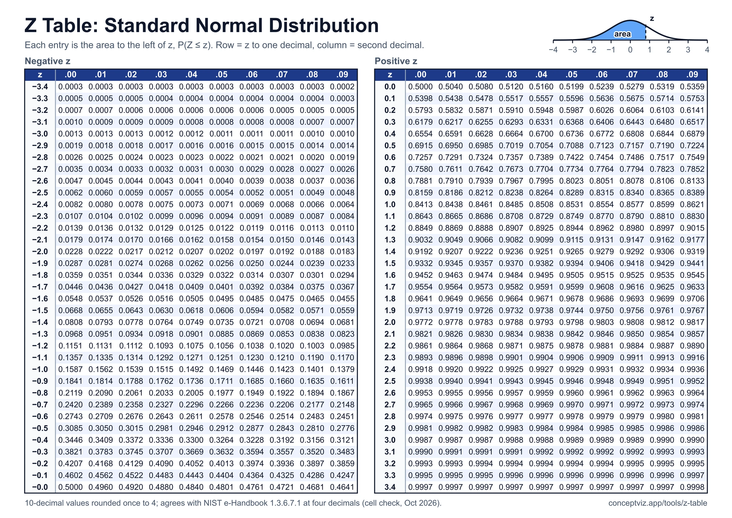
Z table with positive and negative z-scores, left-tail cumulative area, z to p and p to z calculator, shaded curve and printable A4 and Letter sheets.
 Research
Chi-Square Table
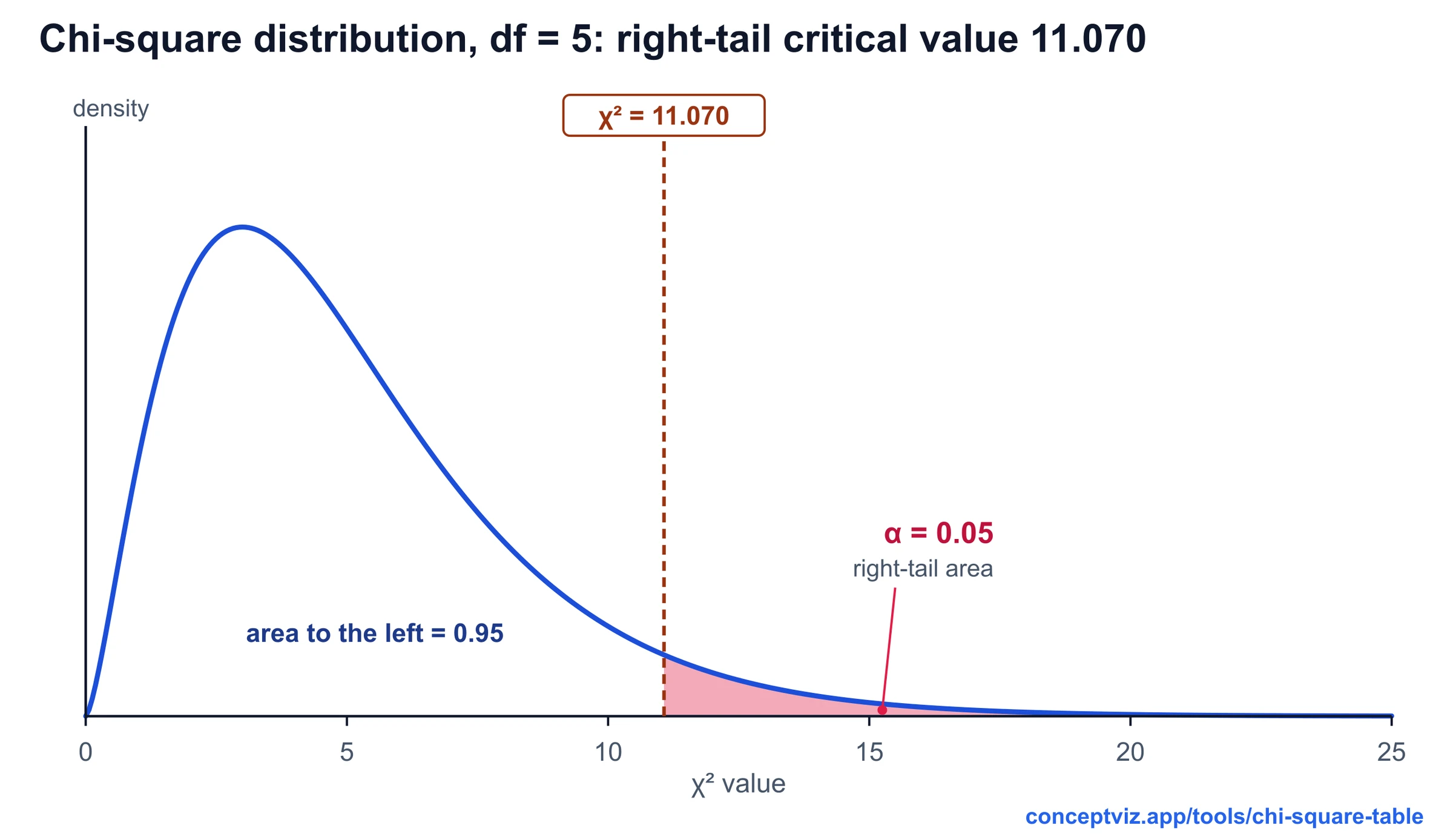
Chi-square table with right-tail critical values for df 1 to 100, a p-value calculator with shaded area and lower-tail columns. Print or download.