Binomial Distribution Table
Binomial distribution table for n = 1 to 20 and 25: individual P(X = k) and cumulative P(X ≤ k), plus a calculator up to n = 1000. Printable.
Binomial probability calculator
Plot these probabilities as a bar chart
P(X = 5)
0.2461
P(X ≤ 5)
0.6230
P(X ≥ 5)
0.6230
P(X < 5)
0.3770
P(X > 5)
0.3770
Mean np
5
Variance np(1 − p)
2.5
Standard deviation
1.58114
Chart style
Binomial probability tables, n = 1 to 20 and 25
Choose n, then read down to k and across to p. The first tab gives the probability of exactly k successes, the second the probability of k or fewer. For p above 0.5, use the symmetry rule under the table.
Number of trials n
Export style
Paper for print
| k \ p | 0.01 | 0.05 | 0.10 | 0.15 | 0.20 | 0.25 | 0.30 | 0.35 | 0.40 | 0.45 | 0.50 |
|---|---|---|---|---|---|---|---|---|---|---|---|
| 0 | |||||||||||
| 1 | |||||||||||
| 2 | |||||||||||
| 3 | |||||||||||
| 4 | |||||||||||
| 5 | |||||||||||
| 6 | |||||||||||
| 7 | |||||||||||
| 8 | |||||||||||
| 9 | |||||||||||
| 10 |
0.0000 means the probability is below 0.00005. It is not exactly zero.
p above 0.5: swap successes and failures. P(X = k; n, p) = P(X = n − k; n, 1 − p), so P(X = 7; n = 10, p = 0.70) is the table entry for k = 3, p = 0.30. For cumulative values, P(X ≤ k; n, p) = 1 − P(X ≤ n − k − 1; n, 1 − p).
Values are rounded half up to four decimals from exact values. We compared every cell with SciPy (binom.pmf and binom.cdf); the only differences are cells exactly on a rounding boundary, such as 0.03125. Click any cell to see it spelled out.
Selected cell
n = 10, p = 0.30, P(X = 3) = 0.2668
More digits: 0.2668.
Free Binomial Distribution Table Charts
Every chart below is drawn from the same code as the tool above. View, download and print them free, no sign-up.
Binomial Distribution Table: P(X = k), n = 10
Exactly-k probabilities for ten trials. For k = 5 and p = 0.50 the entry is 0.2461.
Reference tables
How to read
Distribution
Printable versions
Moving from counts to continuous data? Look up normal areas in the z table, critical values in the t table or the chi-square table, and draw a probability bar chart with the bar chart maker.
What a binomial distribution table shows
- A binomial distribution table lists probabilities for a count of successes. Use it when you repeat the same trial n times and count how many times a result happens: heads in 10 coin flips, defective parts in a batch of 20, correct answers on a multiple-choice quiz.
- The binomial model fits when four conditions hold. There is a fixed number of trials n. Each trial has exactly two outcomes, called success and failure. The probability of success p is the same on every trial. The trials are independent. If you draw without replacement from a small group, the trials are not independent and the binomial is only an approximation.
- The probability of exactly k successes is P(X = k) = C(n, k) p^k (1 − p)^(n − k), where C(n, k) = n! ÷ (k!(n − k)!). The mean is np and the variance is np(1 − p).
How to read the table
- Choose the block for your n, go down to k and across to p. In the individual tab, n = 10, k = 3 and p = 0.30 gives 0.2668, so the chance of exactly 3 successes in 10 trials is 0.2668. In the cumulative tab the same position gives 0.6496, the chance of 3 or fewer. That entry is the sum of the first four individual entries: 0.0282 + 0.1211 + 0.2335 + 0.2668 = 0.6496. The cumulative entry is the exact sum rounded once, so adding rounded entries can occasionally differ in the last digit. Some textbooks print P(X ≥ k) instead of P(X ≤ k), so check the column heading before you read a value.
- A zero in the table is rounded, not exact. With n = 20 and p = 0.05, the chance of no successes is 0.3585, while P(X = 20) shows 0.0000 because it is smaller than 0.00005.
At least, more than, fewer than
- The cumulative tab only answers “k or fewer”, but the other questions are one subtraction away. P(X ≥ k) = 1 − P(X ≤ k − 1). P(X > k) = 1 − P(X ≤ k). P(X < k) = P(X ≤ k − 1). For n = 10 and p = 0.30, the chance of at least 4 successes is 1 − 0.6496 = 0.3504. The calculator at the top of the page gives all five probabilities, P(X = k), P(X ≤ k), P(X ≥ k), P(X < k) and P(X > k), in one go.
When p is greater than 0.5
- The table stops at p = 0.50 because of symmetry. Counting successes with probability p is the same as counting failures with probability 1 − p, so P(X = k; n, p) = P(X = n − k; n, 1 − p). To find P(X = 7) for n = 10 and p = 0.70, look up k = 3 with p = 0.30: 0.2668.
- For cumulative values use P(X ≤ k; n, p) = 1 − P(X ≤ n − k − 1; n, 1 − p). For n = 10, p = 0.70 and k = 7, that is 1 − P(X ≤ 2; n = 10, p = 0.30) = 1 − 0.3828 = 0.6172. If p is not in the table, or n is 21 to 24 or above 25, use the calculator, which accepts any p between 0 and 1 and n up to 1000.
Normal approximation: when it works
- For large n the binomial can be approximated by a normal distribution with mean np and standard deviation √(np(1 − p)). A common rule of thumb asks for np ≥ 10 and n(1 − p) ≥ 10; some textbooks use 5 instead of 10. It is a guideline, not a guarantee.
- Example: n = 100 and p = 0.4 gives np = 40 and n(1 − p) = 60, so the rule is met. The exact P(X ≤ 45) is 0.8689. The normal approximation with a continuity correction, Φ((45.5 − 40) ÷ √24), gives 0.8692. Without the correction, Φ((45 − 40) ÷ √24) gives 0.8463, which is further off. For a z-score lookup, use the z table.
Frequently Asked Questions
Related Statistics Tools
 Research
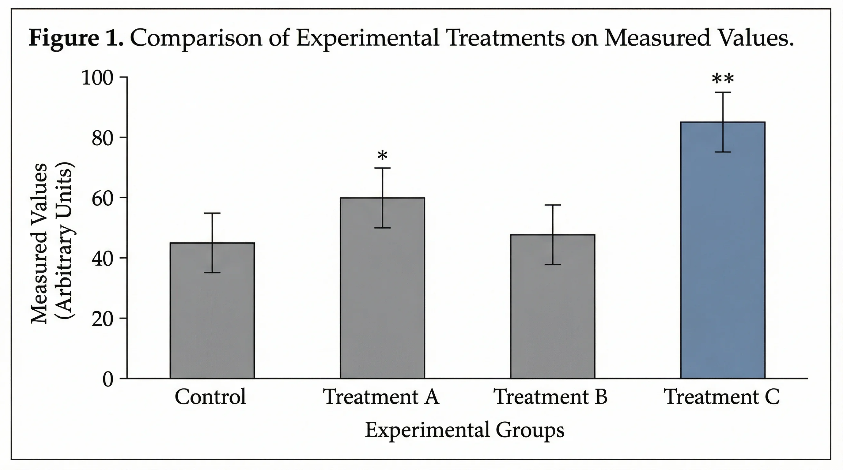
Bar Chart Maker
Create horizontal, grouped, and stacked bar charts for rankings, comparisons, and classroom data visualization.
 Research
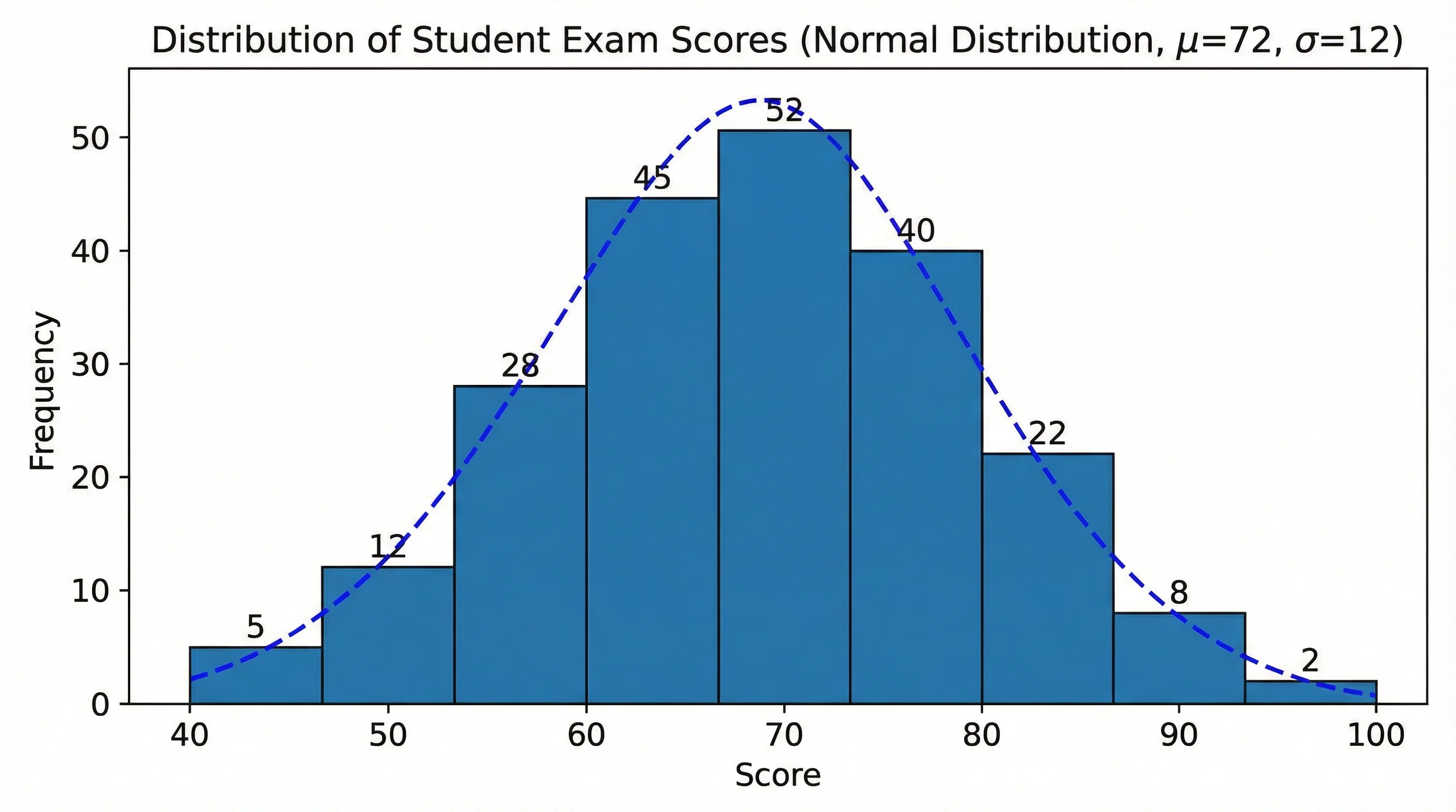
AI Histogram Maker
Create professional histograms and frequency distribution charts for statistics, data analysis, and STEM education.
 Research
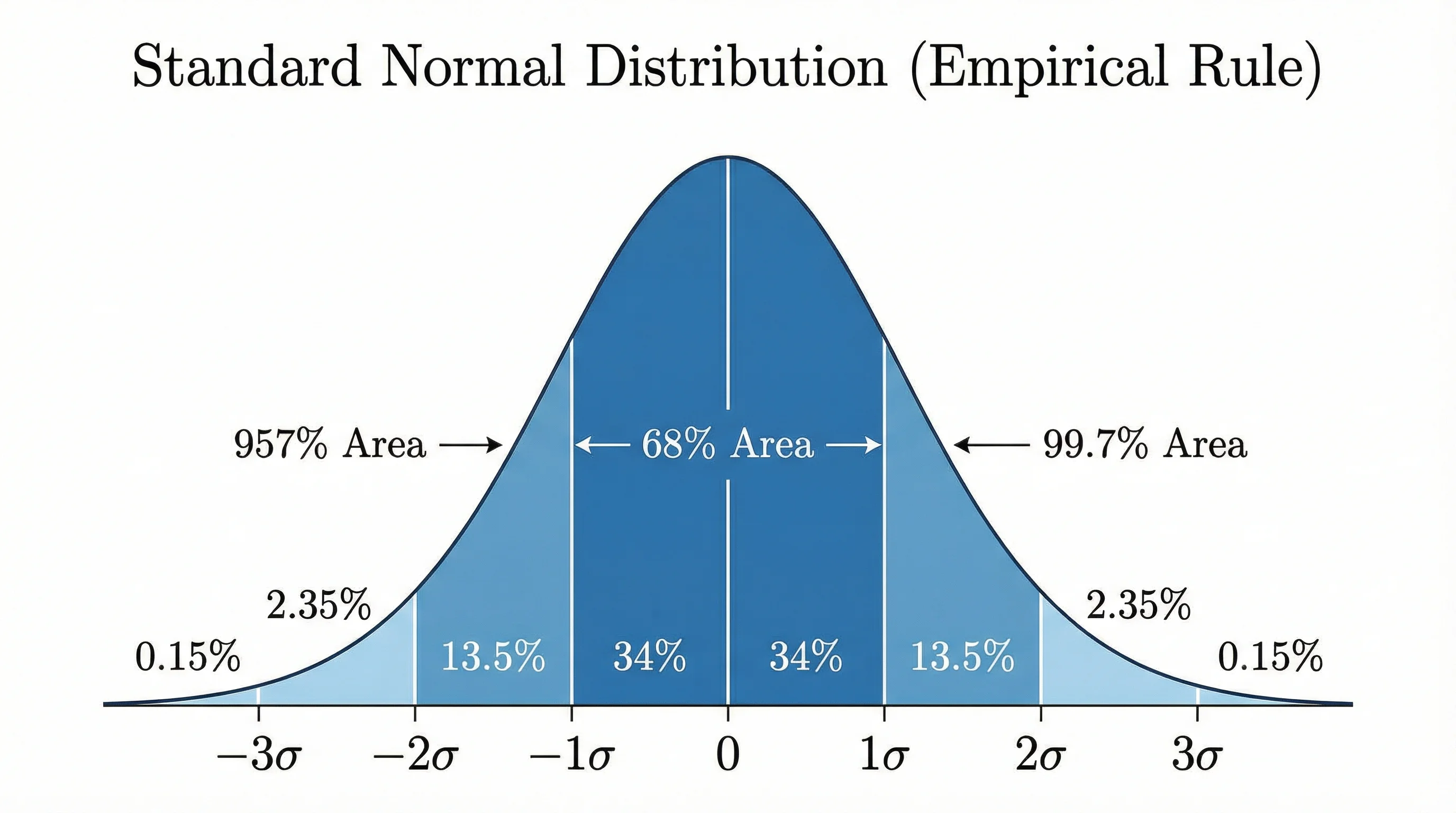
Bell Curve Generator
Create professional bell curves and normal distribution graphs for statistics, data analysis, and academic papers.
 Research
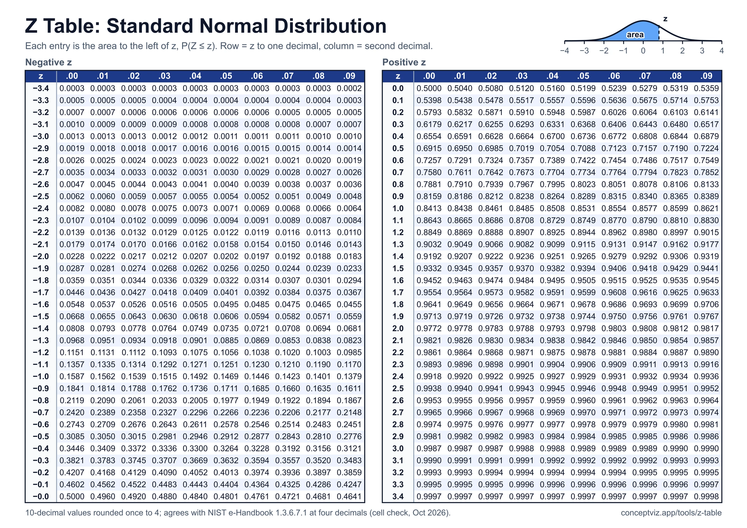
Z Table
Z table with positive and negative z-scores, left-tail cumulative area, z to p and p to z calculator, shaded curve and printable A4 and Letter sheets.
 Research
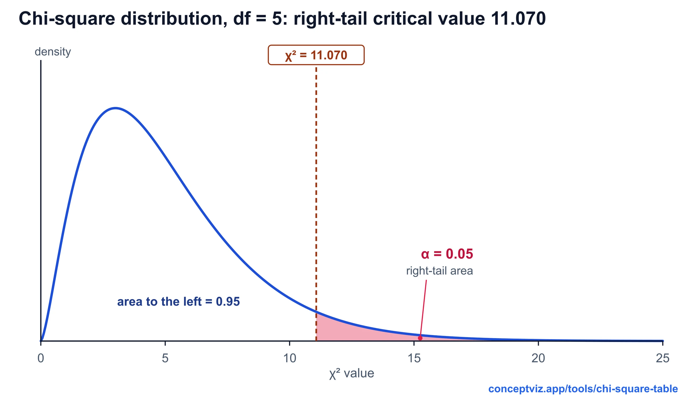
Chi-Square Table
Chi-square table with right-tail critical values for df 1 to 100, a p-value calculator with shaded area and lower-tail columns. Print or download.
 Research
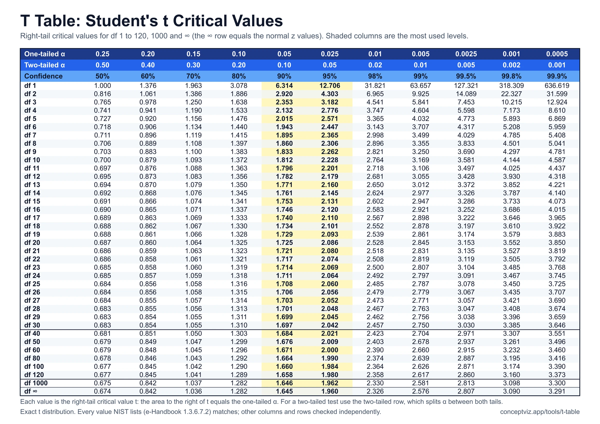
T Table
T table with one-tailed and two-tailed critical values for df 1 to 120 and infinity, a critical value and p-value calculator, and printable sheets.