Effect Size Calculator
Calculate Cohen’s d, Hedges’ g, r and eta squared from means and SDs, t, F, r or odds ratio, with 95% CIs, labels, an overlap chart and an APA sentence. Free.
Need a different curve? Plot a normal curve from any mean and SD in the bell curve generator, or describe two overlapping groups for an illustration.
Open bell curve generator| Measure | Estimate | 95% CI | Cohen (1988) | Sawilowsky (2009) |
|---|---|---|---|---|
| Cohen’s d | 0.333 | [−0.176, 0.843]Exact (non-central t): [−0.178, 0.842] | small | small |
| Hedges’ g | 0.329 | [−0.174, 0.832]Exact (non-central t): [−0.175, 0.831] | small | small |
| r | .167 | [−.089, .394] | small | – |
| η² (= r²) | .028 | [.000, .155] | small | – |
t(58) = 1.291, p = .202, J = 0.9870 (approximation 0.9870), pooled SD = 15.000, mean difference = 5.000
95% CI: estimate ± 1.96 × √V (Hedges & Olkin large-sample variance); the exact line inverts the non-central t distribution. r and η² limits are the d limits passed through the same conversion.
Cohen’s U3
63.1%
above the other mean
Overlap
86.8%
of the curves shared
CL
59.3%
probability of superiority
APA-style sentence
Group 1 (M = 105.00, SD = 15.00) scored higher than Group 2 (M = 100.00, SD = 15.00), t(58) = 1.29, p = .202, Cohen’s d = 0.33, 95% CI [−0.18, 0.84].
Convert between d, r, η² and f
For two groups of equal size: r = d / √(d² + 4), η² = r², f = d / 2.
Cohen’s d
0.500
r
.243
η²
.059
Cohen’s f
0.250
Odds ratio
2.48
Overlap
80.3%
Free Effect Size Charts
Every chart below is drawn from the same code as the calculator above. View and download them free, no sign-up.
Cohen’s d = 0.5: Overlapping Normal Curves
A medium effect drawn as two groups: most of the area is shared, yet the higher group is still ahead on average.
Visual explainers
Reference
Worked examples
Have an effect size and want a sample size? The power analysis calculator turns d, f, r or w into the number of participants you need.
Effect sizes also appear in other tools. The ANOVA table calculator shows η² beside the F test, the correlation coefficient guide covers r, and the t table and F distribution table give the critical values behind the tests. For a visual of the significance region, try the rejection region diagram maker.
What an effect size tells you
A p-value says whether an effect is distinguishable from zero given your sample. It does not say how big the effect is: with enough participants a trivial difference becomes significant, and with too few a large one does not. An effect size answers the other question. Standardized effect sizes such as Cohen’s d, Hedges’ g, r and η² express a difference or a relationship in units that do not depend on the scale you measured, so results from different studies can be compared and combined in a meta-analysis. Journals such as those following the APA guidelines expect you to report one together with a confidence interval.
How to calculate Cohen’s d from means and SDs
- For two independent groups, d is the difference between the means divided by the pooled standard deviation: d = (M1 − M2) / s_pooled, where s_pooled = √[((n1 − 1)·s1² + (n2 − 1)·s2²) / (n1 + n2 − 2)].
- Take two groups of 30 with means 105 and 100 and a standard deviation of 15 in both. The pooled SD is 15.0, so d = 5 / 15.0 = 0.333. The t statistic for the same data is 1.291 with 58 degrees of freedom, and r = .167. The 95% interval for d runs from −0.176 to 0.843, so a difference this size cannot be told from zero with groups of this size.
Hedges’ g: the small-sample correction
Cohen’s d overestimates the population effect a little when samples are small. Hedges’ g multiplies d by a correction factor J that depends on the degrees of freedom: J = Γ(df/2) / (√(df/2) · Γ((df − 1)/2)). The calculator uses this exact factor rather than the common shortcut 1 − 3/(4·df − 1); the two agree to about three decimals. With df = 18, J = 0.9576, a 4% reduction. With df = 58 it is 0.9870, and with df = 398 it is 0.9981, so for large samples g and d are practically the same number. Report g when your groups are small, and say which one you report.
d, d_z and d_av: which standardizer?
In a within-subjects design there is more than one defensible d. d_z divides the mean difference by the standard deviation of the difference scores; it equals t / √n, so you can get it from a paired t test, but it grows when the two measurements are highly correlated. d_av divides by the average of the two standard deviations, which makes it comparable with d from a between-subjects study. The Means & SDs tab reports both when you choose the paired design, and the t value tab reports d_z, the only one that t and n alone can give. Whichever you use, name it in your write-up (Lakens, 2013).
Confidence intervals: large-sample and exact
The main interval uses the large-sample variance of d from Hedges and Olkin (1985), V = (n1 + n2) / (n1·n2) + d² / (2(n1 + n2)), and the limits are the estimate ± 1.96 × √V. It is quick and usually close. The line below it inverts the non-central t distribution: it finds the effect sizes for which your t statistic would sit at the 2.5th and 97.5th percentile. This is the interval to prefer for small samples, and for large d where the symmetric interval becomes too narrow on one side. For F tests the interval for partial η² comes from the non-central F distribution in the same way.
Is 0.4 a good effect size? What do 0.2 and 0.8 mean?
Cohen (1988) suggested 0.2, 0.5 and 0.8 as small, medium and large for behavioural science, and Sawilowsky (2009) added 0.01 very small, 1.2 very large and 2.0 huge. These are rules of thumb for when nothing better is known, not standards. A d of 0.2 means the group means are one fifth of a standard deviation apart: the overlap is 92%, and a random person from the higher group beats a random person from the other group about 56% of the time. A d of 0.8 gives 69% overlap and about 71%. A d of 0.4 sits between small and medium, and in education research it is famous as the “hinge point” that Hattie (2009) proposed as the average effect of a school intervention, a figure that critics argue should not be applied to every study. Whether 0.4 is good depends on the cost of the intervention, the outcome measure and what similar studies find in your field.
Effect size from t, F, r or an odds ratio
- From a t test, d = t × √(1/n1 + 1/n2) for independent groups, so t = 2.5 with 20 per group gives d = 0.791 and g = 0.775. From an F test, partial η² = F·df1 / (F·df1 + df2): F(2, 57) = 4.2 gives .128, with Cohen’s f = 0.384. From a correlation, d = 2r / √(1 − r²), so r = .3 corresponds to d = 0.629 for two equal groups. From an odds ratio, d = ln(OR) × √3 / π (Chinn, 2000).
- Only the t and F routes are exact for the design they came from; the r and odds ratio routes are conversions that assume equal groups and a logistic or normal latent variable, so treat them as approximations.
Using the effect size to plan your next study
Once you have an effect size from a pilot or from the literature, you can ask how many participants a new study needs to detect it. Use the power analysis calculator for that, and shrink published effects a little before you plan around them, because published estimates tend to be inflated. The benchmark table above gives a feel for what an effect looks like, and the related pages explain how the same measures appear in ANOVA output and in correlation tables.
Frequently Asked Questions
Related Statistics Tools
 Research
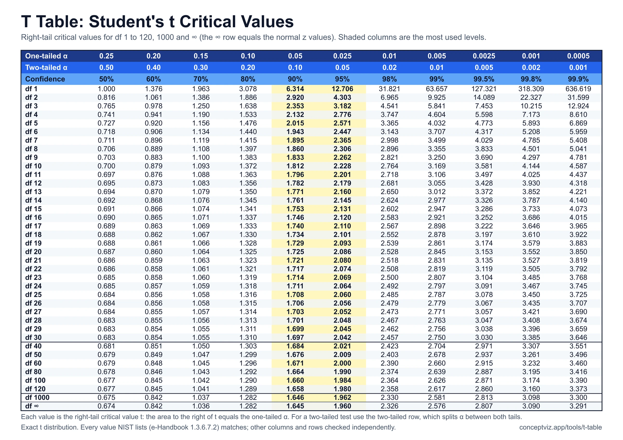
T Table
T table with one-tailed and two-tailed critical values for df 1 to 120 and infinity, a critical value and p-value calculator, and printable sheets.
 Research
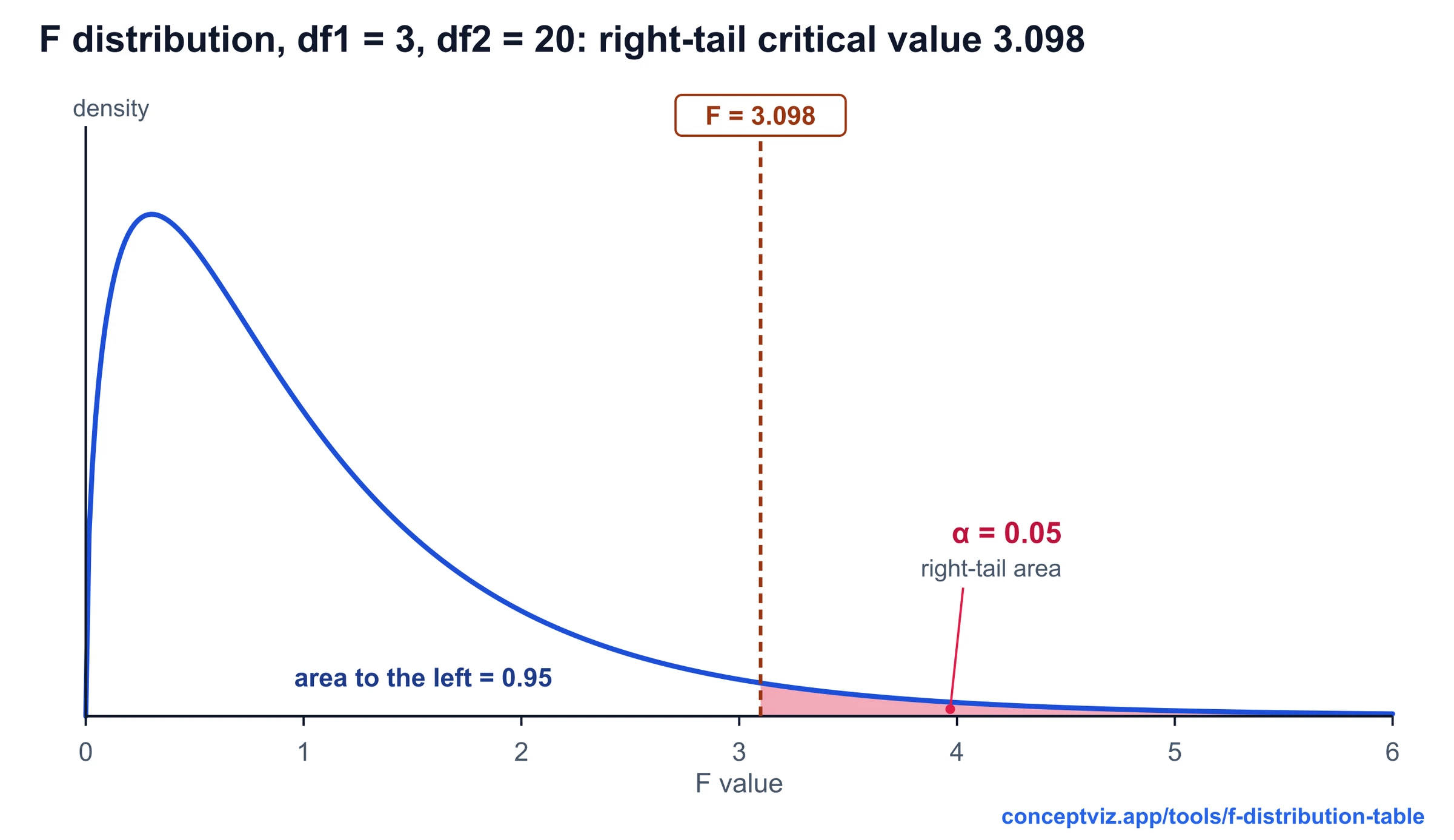
F Distribution Table
F distribution table with right-tail critical values for alpha 0.10, 0.05, 0.025 and 0.01, a critical value and p-value calculator, and printable sheets.
 Research
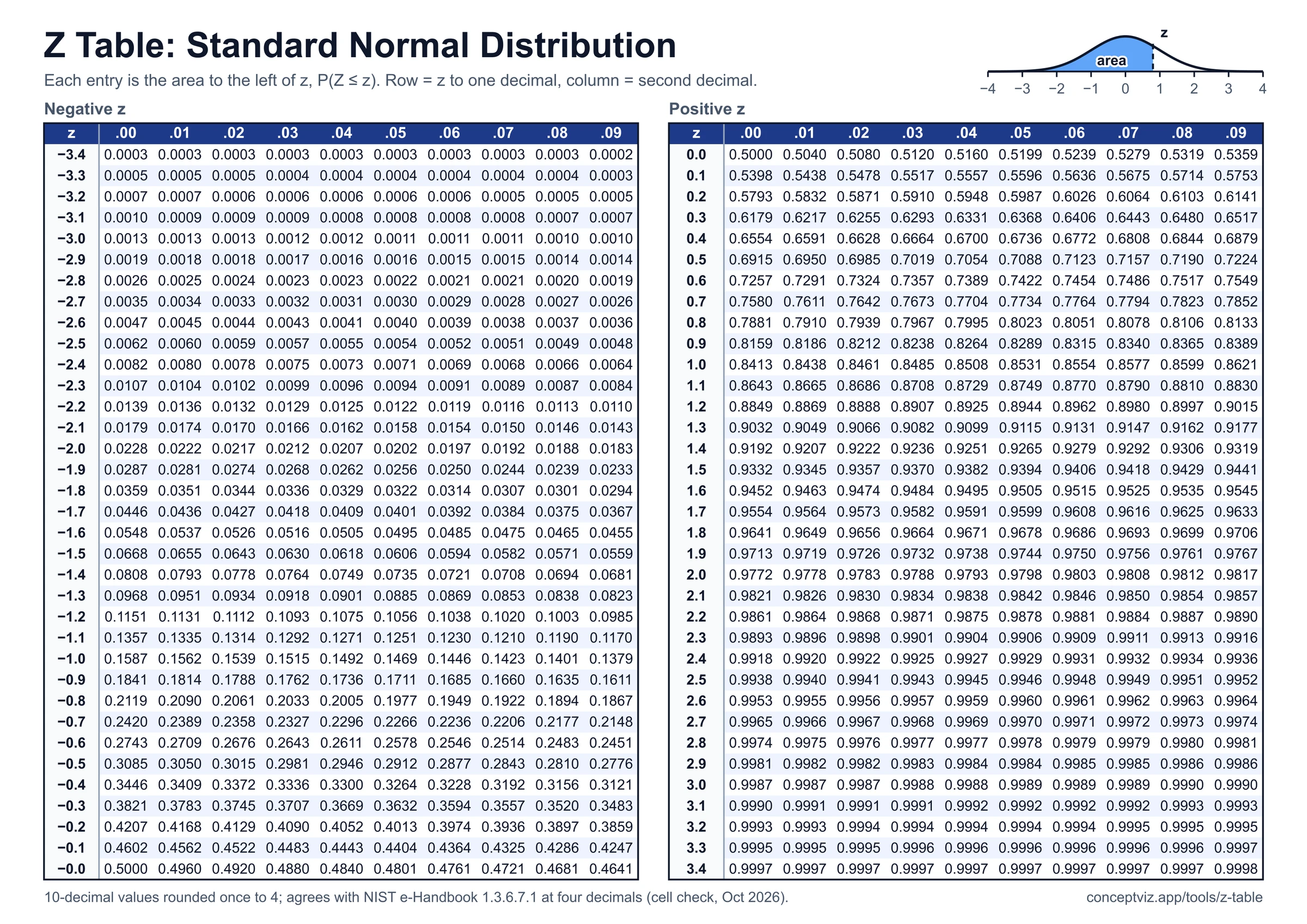
Z Table
Z table with positive and negative z-scores, left-tail cumulative area, z to p and p to z calculator, shaded curve and printable A4 and Letter sheets.