Correlation Coefficient Interpretation
Interpret Pearson r with Cohen, Evans, Dancey & Reidy, Quinnipiac and Chan scales side by side. Get r squared, p, a 95% CI and the APA line.
Add n for the p value and the 95% interval.
| Scale | Label for |r| = .45 |
|---|---|
| Cohen (1988)Behavioral sciences | Medium |
| Evans (1996)Behavioral sciences | Moderate |
| Dancey & ReidyPsychology | ModerateBetween two listed points that share this label (.4 Moderate and .5 Moderate) |
| Quinnipiac UniversityPolitics | StrongBetween two listed points that share this label (.4 Strong and .5 Strong) |
| Chan (2003)Medicine | Fair |
Direction
Positive
The variables rise together
r squared
20.25%
Shared variance
p (two-tailed, df = 28)
.013
t
2.666
95% CI for r
[.11, .70]
Fisher z
APA 7 style write-up
r(28) = .45, p = .013
With the interval: r(28) = .45, p = .013, 95% CI [.11, .70]
p to three decimals, no zero before the decimal point. Statistic symbols are italic when you paste into your paper.
An illustration of what this r looks like, not your data.
Correlation coefficient interpretation chart
Strength labels for the absolute value of r under five published scales. The sign only gives the direction. Dancey and Reidy and Quinnipiac University are printed at steps of 0.1, so values between two rows get a label only when both neighbouring rows share one, and otherwise no label in those scales. Chan has no row for .5 to .6.
| |r| | Cohen (1988)Behavioral sciences | Evans (1996)Behavioral sciences | Dancey & ReidyPsychology | Quinnipiac UniversityPolitics | Chan (2003)Medicine |
|---|---|---|---|---|---|
| 0 | Below small | Very weak | Zero | None | Poor |
| ±.10 | Small | Very weak | Weak | Negligible | Poor |
| ±.20 | Small | Weak | Weak | Weak | Poor |
| ±.30 | Medium | Weak | Weak | Moderate | Fair |
| ±.40 | Medium | Moderate | Moderate | Strong | Fair |
| ±.50 | Large | Moderate | Moderate | Strong | Fair |
| ±.60 | Large | Strong | Moderate | Strong | Moderately strong |
| ±.70 | Large | Strong | Strong | Very strong | Moderately strong |
| ±.80 | Large | Very strong | Strong | Very strong | Very strong |
| ±.90 | Large | Very strong | Strong | Very strong | Very strong |
| ±1 | Large | Very strong | Perfect | Perfect | Very strong |
Cohen (1988) (Behavioral sciences)
- r at or above .10: small
- r at or above .30: medium
- r at or above .50: large
- Below .10: no label (below the small benchmark)
Cohen (1988), benchmarks as restated in Cohen (1992), Table 1.
Checked against Table 1 of Cohen (1992), Psychological Bulletin 112(1), 155-159, which gives r = .10, .30 and .50. The 1988 book was not opened.
Evans (1996) (Behavioral sciences)
- .00 to .19: very weak
- .20 to .39: weak
- .40 to .59: moderate
- .60 to .79: strong
- .80 to 1.0: very strong
Evans (1996), Straightforward Statistics for the Behavioral Sciences.
Taken from two secondary sources that agree (MHS technical manual and the R effectsize documentation). The book was not opened.
Dancey & Reidy (Psychology)
- .1, .2, .3: weak
- .4, .5, .6: moderate
- .7, .8, .9: strong
- 0: zero; 1: perfect
Dancey & Reidy (2007), as printed in Akoglu (2018), Table 1.
Taken from Akoglu (2018), Table 1 (PMC6107969), which prints it at steps of 0.1. The book was not opened.
Quinnipiac University (Politics)
- .1: negligible; .2: weak; .3: moderate
- .4, .5, .6: strong
- .7, .8, .9: very strong
- 0: none; 1: perfect
Political Science Department, Quinnipiac University, as printed in Akoglu (2018), Table 1.
Taken from Akoglu (2018), Table 1 (PMC6107969), which prints it at steps of 0.1. The original was not opened.
Chan (2003) (Medicine)
- At least 0.8: very strong
- 0.6 up to 0.8: moderately strong
- 0.3 to 0.5: fair
- Less than 0.3: poor
- Nothing between 0.5 and 0.6
Chan (2003), Singapore Medical Journal 44(12), Table II.
Read from Table II of the article itself (PDF). It is the only one of the five checked in its original source.
What different values of r look like
Each panel plots the same 60 x values, so only the spread around the line changes. The plotted points are fixed, and the sample r computed from each panel equals its label.
Direction
r squared: how much variance is shared
Squaring r gives the share of variance in common. No strength labels are given for r squared here: what counts as large depends on the field.
Same r, different data: Anscombe's quartet
Four data sets with a correlation of about .816 each. Only the first looks like the story r tells.
Free Correlation Interpretation Charts
Every chart below is drawn from the same code as the tool above. View, download and print them free, no sign-up.
Correlation Coefficient Interpretation Chart
The same r under five published scales, with the boundaries as printed.
Reference charts
What r looks like
Pitfalls
Worked examples
To check whether a sample r is significant, read the Pearson r column of the critical values table or turn it into a p value with the p-value table. To plot your own pairs, use the scatter plot maker. To compare group means instead of relating two variables, see the ANOVA table and the Tukey table.
How to interpret a correlation coefficient
- Pearson r answers three separate questions, and each one needs its own check. Direction comes from the sign: a positive r means the two variables rise together, a negative r means one falls as the other rises. Strength comes from the size of |r|, from 0 (no linear relationship) to 1 (all points on a straight line). Significance comes from the p value, which depends on both r and the sample size n. A reader who mixes these up will call a tiny effect important or a large one unreliable.
- Strength labels are conventions, not laws. Several published scales exist and they do not agree, so the calculator above shows them side by side and the table below lists every boundary. Pick the scale used in your field or by your instructor, cite it, and say which one you used.
The Pearson r formula
- Pearson r is r = Σ(x − x̄)(y − ȳ) / √[Σ(x − x̄)² × Σ(y − ȳ)²]: how much x and y vary together, divided by how much each varies alone. It always falls between −1 and 1 and does not change when you shift or stretch either variable by a positive factor (a negative factor flips the sign). A small check: x = 1, 2, 3, 4, 5 and y = 2, 4, 5, 4, 5 give r = .775.
Why five scales give five answers
- Cohen (1988) proposed r = .10, .30 and .50 as small, medium and large effects for the behavioral sciences, restated in Cohen (1992). He gave three benchmark values, not intervals; this page reads them as "at or above" cut-offs and says so. Evans (1996) splits |r| into five bands of width .20, from very weak below .20 to very strong from .80. Dancey and Reidy (psychology) and the Quinnipiac University political science scale are printed at steps of 0.1, so between two listed points they give a label only when both neighbouring points share one, and otherwise no label. Chan (2003), written for medical readers, is the most cautious: nothing below .30 is better than poor, and the labels jump from fair (.3 to .5) to moderately strong (.6 to .8) with no row for .5 to .6.
- The same value therefore changes name. An r of .70 is strong in Evans and in Dancey and Reidy, very strong at Quinnipiac, large for Cohen and only moderately strong in Chan. Compare the scales in the chart rather than quoting one label out of context.
Is 0.7 a good correlation? Is 0.3? What does 0.8 mean?
- There is no universal answer; it depends on the field and on the scale you cite. For r = .30, the labels are: Cohen (1988): medium; Evans (1996): weak; Dancey & Reidy: weak; Quinnipiac University: moderate; Chan (2003): fair. For r = .70: Cohen (1988): large; Evans (1996): strong; Dancey & Reidy: strong; Quinnipiac University: very strong; Chan (2003): moderately strong. For r = .80: Cohen (1988): large; Evans (1996): very strong; Dancey & Reidy: strong; Quinnipiac University: very strong; Chan (2003): very strong.
- Whether a value is good also depends on what you need it for. A reliability coefficient or a calibration line is usually expected to be well above .90. A relationship between two human behaviors rarely reaches .50, so .30 can be a meaningful finding there. Judge r against what earlier studies in your area report.
r squared interpretation
- Squaring r gives the proportion of variance the two variables have in common, which Chan (2003) calls the coefficient of determination. It is not a stronger or weaker version of r, and the labels written for r do not transfer to it: r = .30 shares 9% of the variance, r = .50 shares 25% and r = .70 shares 49%. The chart above gives the full table from r = .1 to 1.
- In regression, R² is the share of the variation in the outcome that the model explains. What counts as a high R² depends on the domain. A physical calibration with controlled conditions is expected to explain nearly all the variation. A model of human behavior, health or markets can be useful with a much smaller share, because many other factors are not in the model. This page gives no cut-offs for r squared on purpose: report the value, compare it with similar studies, and judge it against what the model is for.
Significant does not mean strong
- The p value tests whether r differs from zero, using t = r√(n − 2) / √(1 − r²) with n − 2 degrees of freedom. With a large sample a small r becomes significant: r = .10 with n = 400 gives t = 2.01 and p = .046, yet r squared is only 1% and every scale on this page puts it at the bottom of its range (small, very weak, weak, negligible or poor). Report the 95% interval as well. It comes from the Fisher z transformation: z′ = atanh(r), a standard error of 1 / √(n − 3), then tanh back to the r scale. For r = .45 with n = 30 the interval is [.11, .70], wide enough to show how uncertain a small sample is.
A negative example
- Suppose r = −.55 with n = 12. The sign says that one variable falls as the other rises. Strength is |r| = .55, which gives: Cohen (1988): large; Evans (1996): moderate; Dancey & Reidy: moderate; Quinnipiac University: strong; Chan (2003): no label. The test gives r(10) = −.55, p = .064, 95% CI [−.85, .03], so the interval reaches past zero and the sample is too small to rule out no correlation. The sign never changes the strength label: r = −.55 is as strong as r = .55.
How to read a correlation matrix table
- Software often prints many correlations at once as a square table, one row and one column per variable. The diagonal is always 1, because each variable correlates perfectly with itself. The cell for A and B equals the cell for B and A, so the upper and lower triangles repeat each other and you only need to read one of them. Each cell can carry its own p value and n, and the n can differ between cells when missing values are dropped pair by pair. Read each cell as a separate r: give its sign, its strength with the scale you chose, and its interval. With many cells some will pass p < .05 by chance, so treat a lone significant cell in a large table with caution and consider a correction for multiple tests.
Effect size: r and Cohen's d
- r is itself an effect size, and the benchmarks .10, .30 and .50 apply to r. Cohen's d has its own benchmarks, .2, .5 and .8, so the two sets of cut-offs cannot be swapped. For two groups of equal size r = d / √(d² + 4), which turns d = .2, .5 and .8 into r = .10, .24 and .37. This is a standard conversion, not a quotation from Cohen, and it assumes equal group sizes.
Correlation is not causation, and r can mislead
- A correlation says that two variables move together. It does not say that one causes the other: a third variable, reverse causation or chance can produce the same r. Pearson r also measures only straight-line association. A curve can have r near zero, one outlier can create or erase a correlation, and a restricted range lowers it. Anscombe's quartet shows four data sets with almost the same r of about .816 and four different stories, so plot the data before you interpret the number.
- When the relationship is monotonic but not linear, or the data are ranks or contain strong outliers, Spearman rank correlation is the usual alternative. It is Pearson r computed on the ranks, and the same labels are often applied to both. In simple linear regression with one predictor, R² equals r².
How to report a correlation in APA style
- APA 7 reports r with its degrees of freedom (n − 2), no zero before the decimal point for r and p, and exact p to three decimals unless p is below .001. Example: r(28) = .45, p = .013. With the interval: r(28) = .45, p = .013, 95% CI [.11, .70]. Name the correlation (Pearson or Spearman), give the direction in words, and add a plain-language description of the strength with the scale you used.
Frequently Asked Questions
Related Statistics Tools
 Research
Scatter Plot Maker
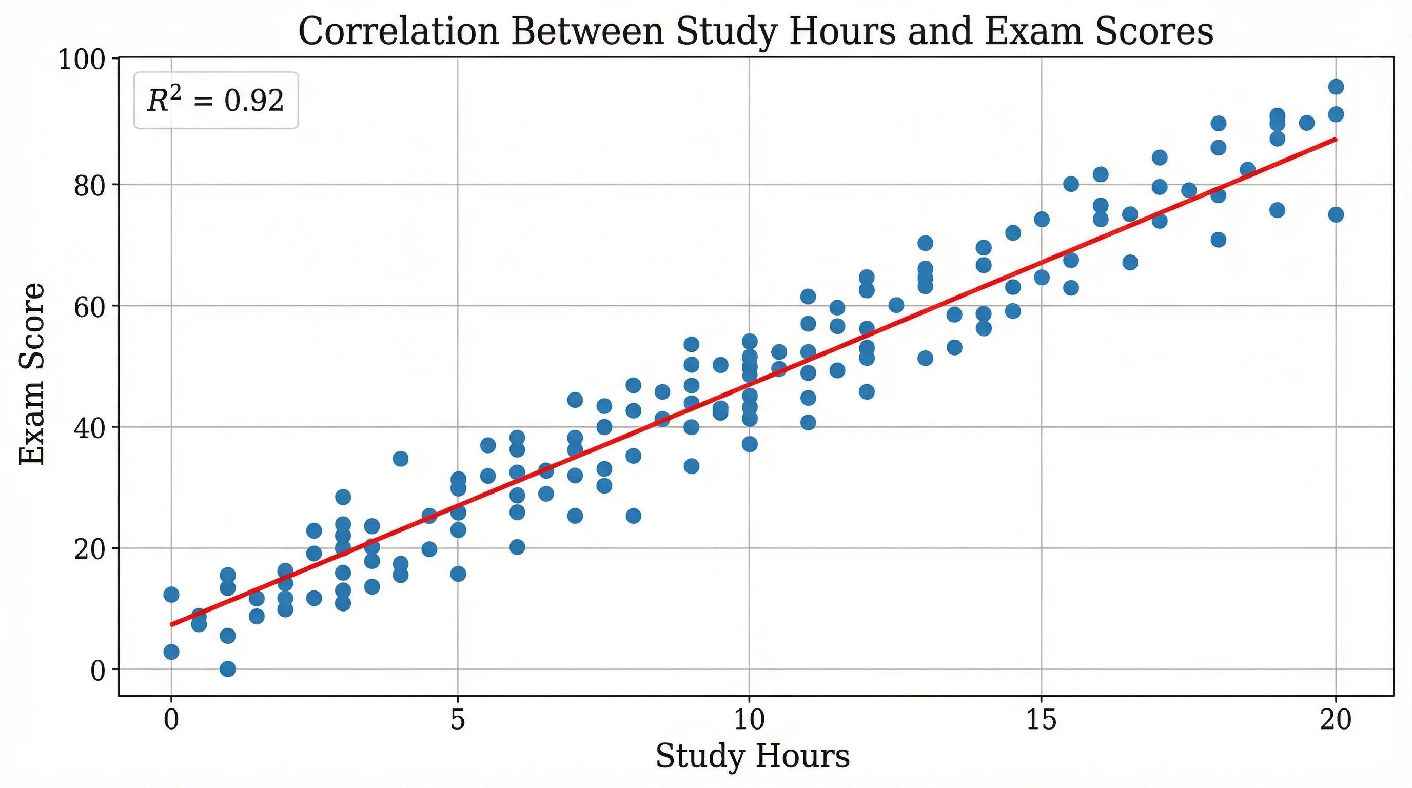
Paste X,Y pairs to draw a scatter plot with a line of best fit and the Pearson r value, then download the SVG.
 Research
Critical Values Table
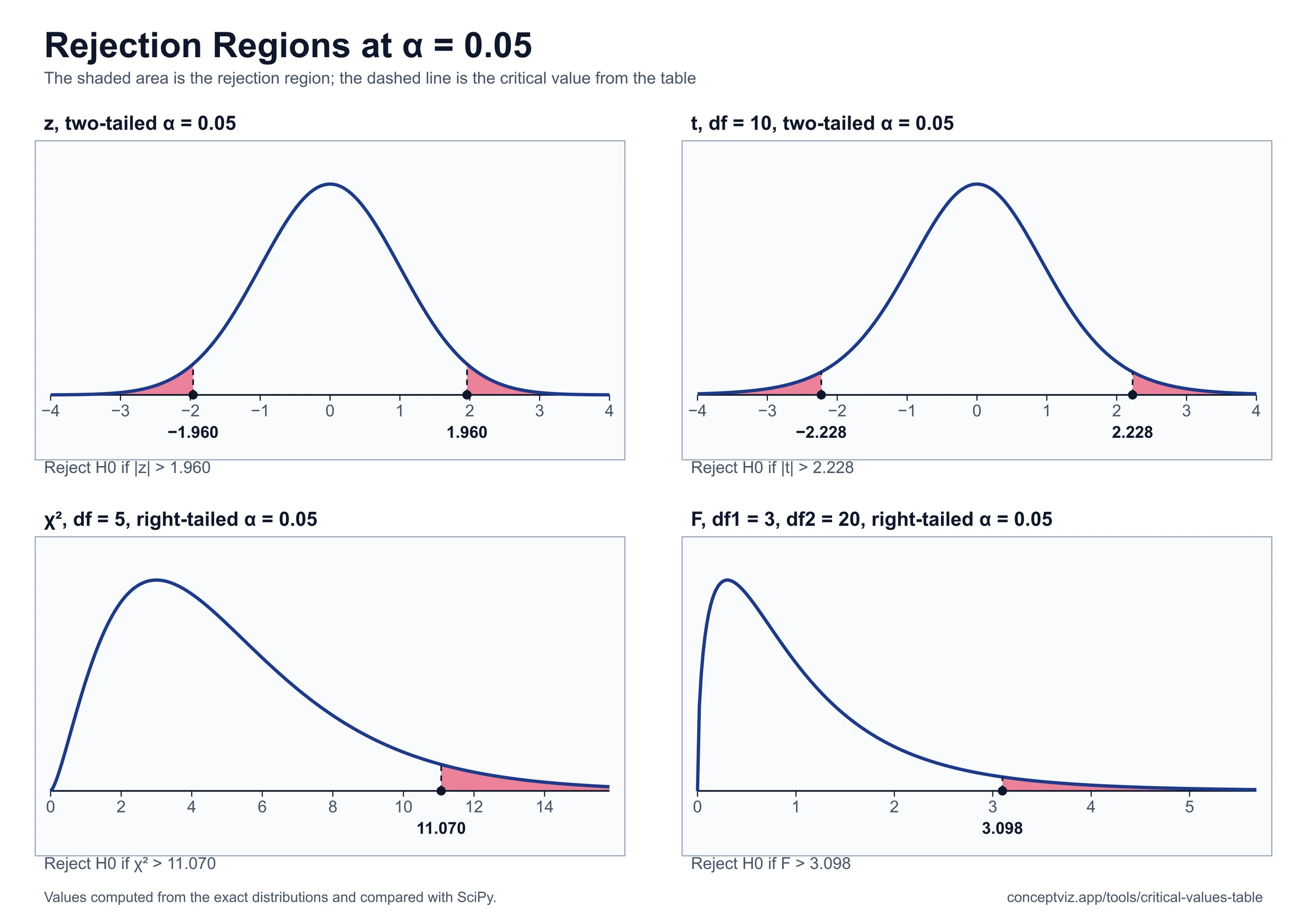
Critical values table for z, t, chi-square, F and Pearson r: enter alpha and df to get the value, with quick tables and a printable r table.
 Research
P-Value Table
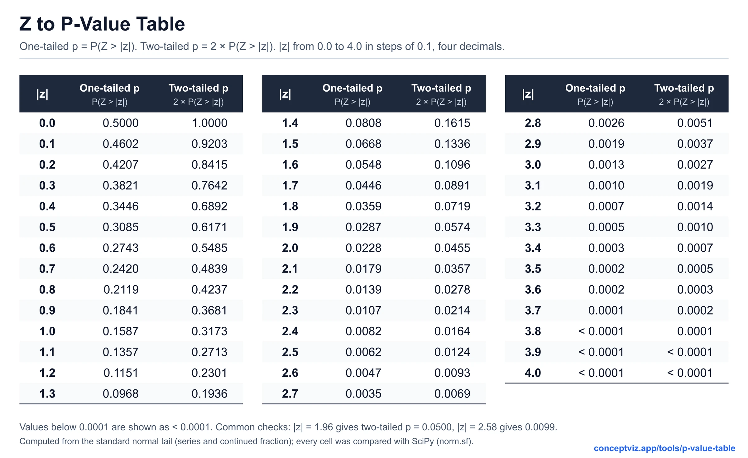
Turn a z, t, chi-square, F or r statistic into a p-value and see how to report it in APA style.