Tukey Table (Studentized Range q)
Tukey table of studentized range q critical values for alpha 0.10, 0.05 and 0.01, k = 2 to 20 groups. Look up q, compute Tukey HSD and compare group means.
Significance level α
Total observations minus k in a one-way ANOVA.
Critical studentized range
q(0.05; k = 3, df = 10) = 3.877
Read directly from the table (this cell is highlighted in the export).
Exports the full α = 0.05 table.
Free Tukey Table Charts
Every chart below is drawn from the same code as the tool above. Download any table as PNG or SVG, or use the Print button and choose Save as PDF in your browser. Free, no sign-up.
Tukey Table: Alpha 0.05
The most used Tukey table: critical q at the 5% level for 2 to 20 groups and df 1 to infinity.
Reference tables
Printable versions
How to read
Worked examples
Tukey’s test comes after a significant F test, so start with the ANOVA table and its F distribution table. For two groups only, a t table is enough, and the critical values table puts z, t, chi-square, F and r cut-offs side by side. For reading correlations rather than group differences, see correlation coefficient interpretation.
What the studentized range is
The studentized range q is the gap between the largest and the smallest of k sample means, divided by the standard error of a mean. Its distribution depends on two numbers: k, the number of groups being compared, and the error degrees of freedom. Because it looks at the biggest possible gap among all k means, a critical q already accounts for the fact that you are comparing many pairs at once. That is what keeps the familywise error rate at α, and it is why q values grow as k grows, unlike a single t critical value.
When to use a Tukey test
Use Tukey’s honestly significant difference (HSD) test to compare every pair of group means. It is usually run after a one-way ANOVA: the ANOVA F test says whether the means are all equal, and Tukey says which pairs differ. Tukey’s procedure itself controls the familywise error rate at α, so it does not depend on the F test being significant. It works best when groups are the same size, and the error df and MSW come straight from the ANOVA table.
How to read the Tukey table
- Pick the tab for your α, or use the q lookup tab as a Tukey q calculator. Find the column for k, the number of groups, and the row for the error degrees of freedom, which is the total number of observations minus k. The cell where they meet is the critical q. For k = 3, df = 10 and α = 0.05 the cell is 3.877.
- Other cells you can check: q(0.01; 5, 20) = 5.293 and q(0.05; 10, 60) = 4.646. The last row, df = ∞, is the limit for very large samples, for example q(0.05; 2, ∞) = 2.772, which is √2 times the normal critical value 1.96.
Tukey HSD calculator: formula and worked example
- For groups of equal size n, the honestly significant difference is HSD = q × √(MSW / n), where MSW is the within-groups mean square from the ANOVA table. Two group means differ significantly when the absolute difference between them is larger than HSD.
- Take 3 groups of 10 with error df = 27 and MSW = 4.2, at α = 0.05. The table has no row for df = 27, so q is interpolated between the rows for 24 and 30, giving 3.506. Then HSD = 3.506 × √(4.2 / 10) = 2.272. With means of 20.1, 22.9 and 24.3, the Control vs Drug A gap is 2.8 and Control vs Drug B is 4.2, both above 2.27. Drug A vs Drug B is 1.4, which is not.
Unequal group sizes: Tukey-Kramer
When group sizes differ, use the Tukey-Kramer adjustment: for groups i and j the critical difference is q × √((MSW / 2) × (1/ni + 1/nj)). With equal n this reduces to the HSD formula above. The calculator applies it to every pair when you choose unequal n. With unequal sizes the method is conservative: the familywise error rate stays at or below α (see the NIST Engineering Statistics Handbook, section 7.4.7.1). Most statistics packages use this form for unequal group sizes.
If your df is not in the table
Printed tables skip rows between 20 and 120. The usual rule is to interpolate linearly in 1/df between the two neighbouring rows, which is what the calculator does and states on the result. For example, q(0.05; 3, 45) comes out as 3.428, between the df = 40 and df = 60 rows. Interpolation is very close but not exact, so report the exact value from statistical software when you need it. The cautious manual habit is to use the next smaller df, which gives a slightly larger q.
Assumptions and reporting in APA style
- Tukey’s test assumes independent observations, roughly normal residuals within each group and similar variances across groups, the same assumptions as the one-way ANOVA that comes before it. If variances are clearly unequal, Games-Howell is the usual alternative.
- A sentence in APA style looks like this: “Tukey HSD post hoc comparisons showed that the Control group (M = 20.10) scored lower than Drug A (M = 22.90) and Drug B (M = 24.30), both p < .05, while Drug A and Drug B did not differ.” Report exact p-values from your software when you have them; this page compares each difference with the critical value at your α and does not compute exact Tukey p-values.
Frequently Asked Questions
Tukey vs Bonferroni vs Scheffé vs Games-Howell
These are the multiple comparison procedures students meet most often. The summary below follows the usual textbook description, and the NIST e-Handbook covers Tukey, Scheffé and Bonferroni in its section 7.4.7. Games-Howell is described in Games and Howell (1976), listed in the references.
| Method | Best used for | Equal variances needed? | Equal n needed? |
|---|---|---|---|
| Tukey HSD | All pairwise comparisons after a one-way ANOVA | Yes | Exact for equal n; Tukey-Kramer for unequal n |
| Bonferroni | A small set of planned comparisons, each tested at α divided by the number of tests | Yes, when it uses the pooled MSW | No |
| Scheffé | All possible contrasts, not only pairs, such as one group against the average of two others | Yes | No |
| Games-Howell | All pairwise comparisons when group variances look unequal | No | No |
Tukey HSD in Python
To check a value from the table, call SciPy directly. The code below was run with SciPy 1.18.1 and statsmodels 0.15.0.
from scipy.stats import studentized_range
studentized_range.ppf(0.95, 3, 10)   # 3.876777 -> 3.877 in the table

from statsmodels.stats.multicomp import pairwise_tukeyhsd
res = pairwise_tukeyhsd(values, labels, alpha=0.05)
print(res.summary())
Run on three groups of five (4, 5, 6, 5, 4 / 6, 7, 8, 7, 7 / 9, 10, 11, 10, 9), statsmodels reported mean differences of 2.2 (A-B), 5.0 (A-C) and 2.8 (B-C), each with an interval of plus or minus 1.3428, and all three pairs significant. By hand, MSW = 0.6333 with 12 error df, the table gives q(0.05; 3, 12) = 3.773, and HSD = 3.773 × √(0.6333 / 5) = 1.343, the same width. SciPy also offers scipy.stats.tukey_hsd, which returned the same intervals.
References
- Tukey, J. W. (1949). Comparing individual means in the analysis of variance. Biometrics, 5(2), 99-114. doi:10.2307/3001913
- Games, P. A., & Howell, J. F. (1976). Pairwise multiple comparison procedures with unequal n’s and/or variances: A Monte Carlo study. Journal of Educational Statistics, 1(2), 113-125. doi:10.3102/10769986001002113
- NIST/SEMATECH e-Handbook of Statistical Methods, 7.4.7.1 Tukey’s method.
Related Statistics Tools
 Research
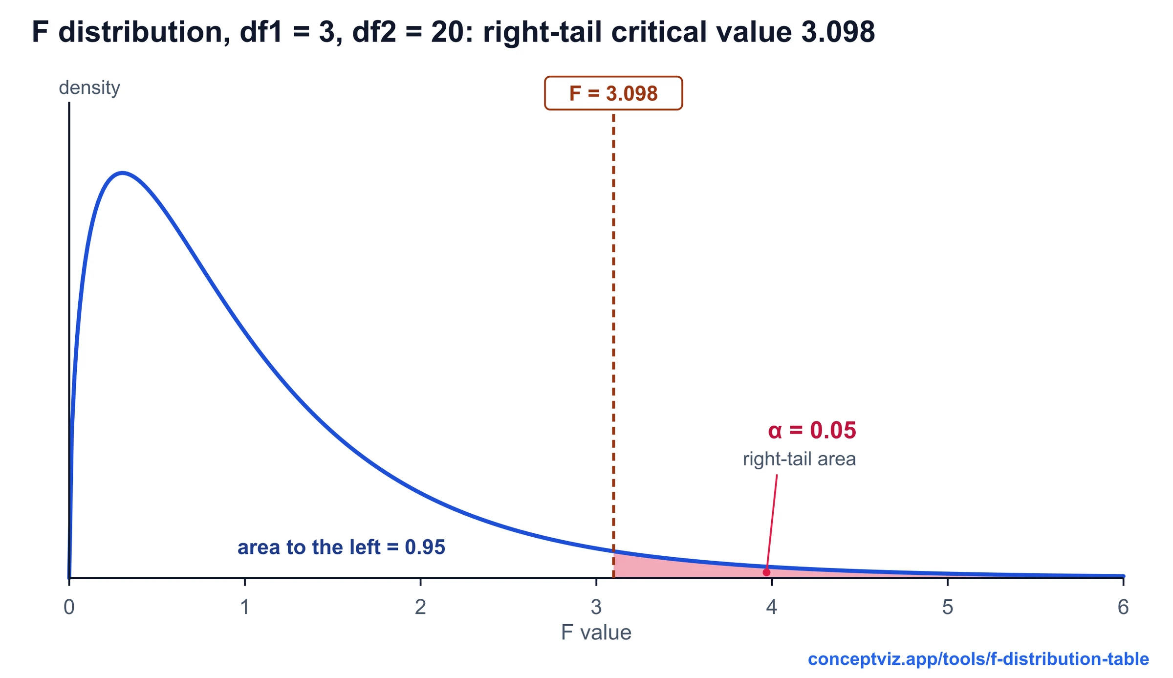
F Distribution Table
F distribution table with right-tail critical values for alpha 0.10, 0.05, 0.025 and 0.01, a critical value and p-value calculator, and printable sheets.
 Research
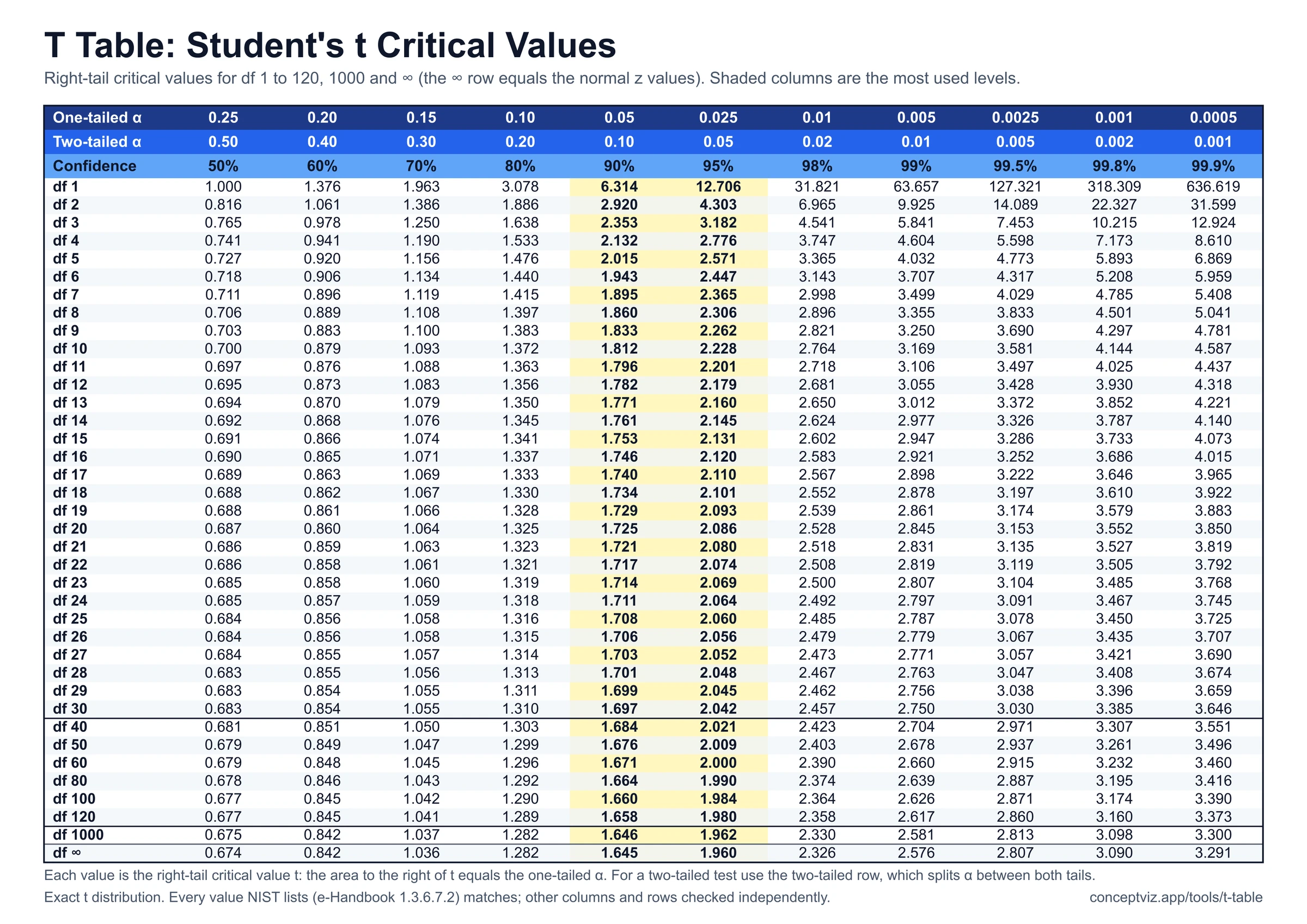
T Table
T table with one-tailed and two-tailed critical values for df 1 to 120 and infinity, a critical value and p-value calculator, and printable sheets.
 Research
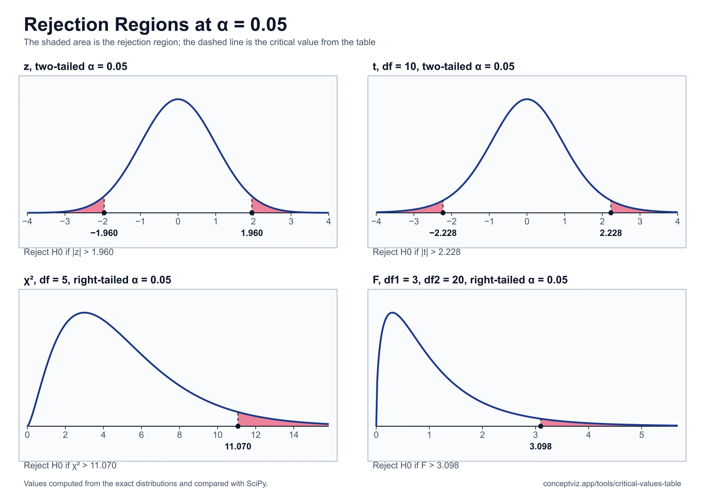
Critical Values Table
Critical values table for z, t, chi-square, F and Pearson r: enter alpha and df to get the value, quick-reference tables and a printable r table.