Critical Values Table
Critical values table for z, t, chi-square, F and Pearson r. Enter alpha and df to get the value, with quick-reference tables and a printable r table.
Distribution
Tail
Type inf for the normal limit.
Critical value
±2.228
Reject H0 if |t| > 2.228
α = 0.05, two-tailed, df = 10.
More digits: -2.228138852 and 2.228138852
Common critical values at a glance
These are the values most coursework asks for. The calculator above gives any other α or df, and the full tables are one click away.
z critical values
Standard normal. For every z-score and area, see the z table.
| Confidence | Two-tailed α | One-tailed α | z |
|---|---|---|---|
| 80% | 0.20 | 0.10 | 1.282 |
| 90% | 0.10 | 0.05 | 1.645 |
| 95% | 0.05 | 0.025 | 1.960 |
| 98% | 0.02 | 0.01 | 2.326 |
| 99% | 0.01 | 0.005 | 2.576 |
| 99.8% | 0.002 | 0.001 | 3.090 |
| 99.9% | 0.001 | 0.0005 | 3.291 |
Chi-square right-tail critical values
Right-tail area α, df 1 to 10, 15, 20 and 30. The chi-square table goes up to df 100.
| df | α = 0.10 | α = 0.05 | α = 0.025 | α = 0.01 |
|---|---|---|---|---|
| 1 | 2.706 | 3.841 | 5.024 | 6.635 |
| 2 | 4.605 | 5.991 | 7.378 | 9.210 |
| 3 | 6.251 | 7.815 | 9.348 | 11.345 |
| 4 | 7.779 | 9.488 | 11.143 | 13.277 |
| 5 | 9.236 | 11.070 | 12.833 | 15.086 |
| 6 | 10.645 | 12.592 | 14.449 | 16.812 |
| 7 | 12.017 | 14.067 | 16.013 | 18.475 |
| 8 | 13.362 | 15.507 | 17.535 | 20.090 |
| 9 | 14.684 | 16.919 | 19.023 | 21.666 |
| 10 | 15.987 | 18.307 | 20.483 | 23.209 |
| 15 | 22.307 | 24.996 | 27.488 | 30.578 |
| 20 | 28.412 | 31.410 | 34.170 | 37.566 |
| 30 | 40.256 | 43.773 | 46.979 | 50.892 |
t critical values
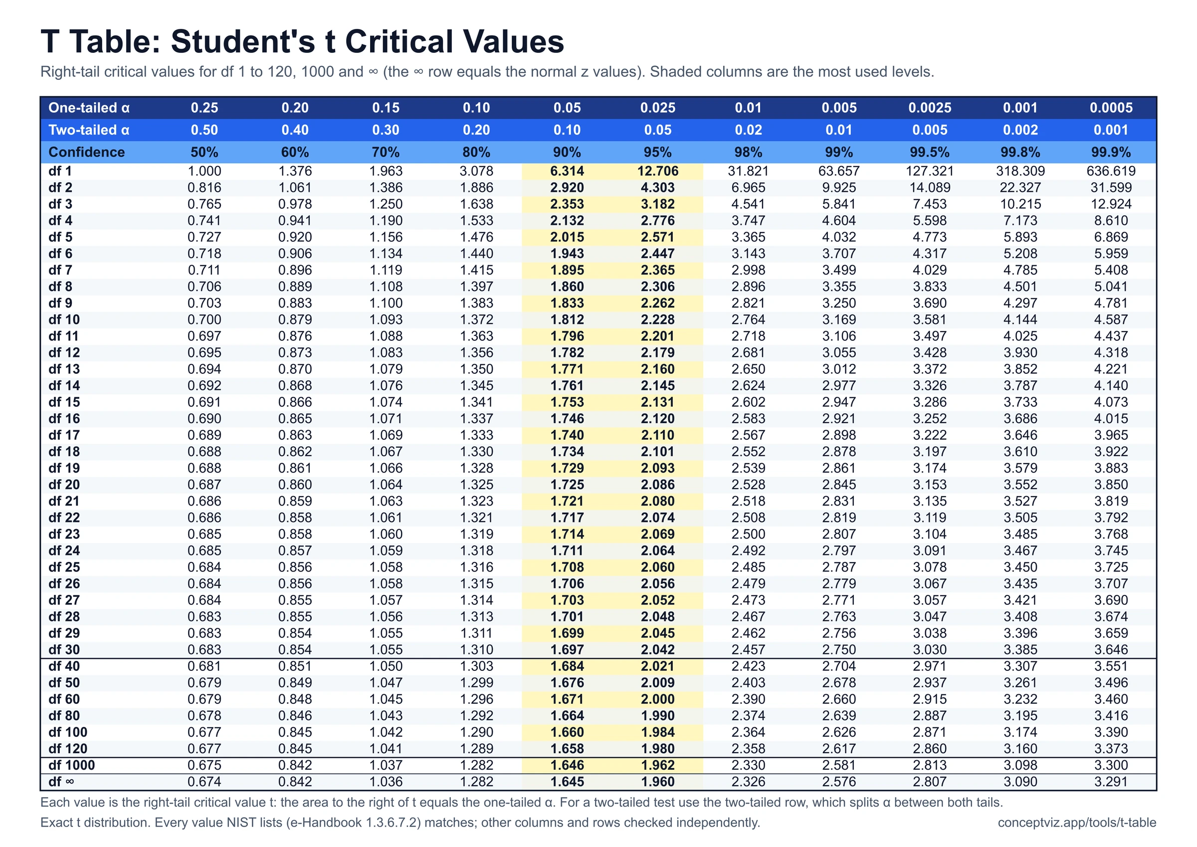
One-tailed α in the top row, two-tailed α below it. The t table lists every df up to 120.
| df | 0.10 | 0.05 | 0.025 | 0.01 | 0.005 | 0.001 | 0.0005 |
|---|---|---|---|---|---|---|---|
| 0.20 | 0.10 | 0.05 | 0.02 | 0.01 | 0.002 | 0.001 | |
| 1 | 3.078 | 6.314 | 12.706 | 31.821 | 63.657 | 318.309 | 636.619 |
| 2 | 1.886 | 2.920 | 4.303 | 6.965 | 9.925 | 22.327 | 31.599 |
| 3 | 1.638 | 2.353 | 3.182 | 4.541 | 5.841 | 10.215 | 12.924 |
| 4 | 1.533 | 2.132 | 2.776 | 3.747 | 4.604 | 7.173 | 8.610 |
| 5 | 1.476 | 2.015 | 2.571 | 3.365 | 4.032 | 5.893 | 6.869 |
| 6 | 1.440 | 1.943 | 2.447 | 3.143 | 3.707 | 5.208 | 5.959 |
| 7 | 1.415 | 1.895 | 2.365 | 2.998 | 3.499 | 4.785 | 5.408 |
| 8 | 1.397 | 1.860 | 2.306 | 2.896 | 3.355 | 4.501 | 5.041 |
| 9 | 1.383 | 1.833 | 2.262 | 2.821 | 3.250 | 4.297 | 4.781 |
| 10 | 1.372 | 1.812 | 2.228 | 2.764 | 3.169 | 4.144 | 4.587 |
| 15 | 1.341 | 1.753 | 2.131 | 2.602 | 2.947 | 3.733 | 4.073 |
| 20 | 1.325 | 1.725 | 2.086 | 2.528 | 2.845 | 3.552 | 3.850 |
| 25 | 1.316 | 1.708 | 2.060 | 2.485 | 2.787 | 3.450 | 3.725 |
| 30 | 1.310 | 1.697 | 2.042 | 2.457 | 2.750 | 3.385 | 3.646 |
| 40 | 1.303 | 1.684 | 2.021 | 2.423 | 2.704 | 3.307 | 3.551 |
| 60 | 1.296 | 1.671 | 2.000 | 2.390 | 2.660 | 3.232 | 3.460 |
| 120 | 1.289 | 1.658 | 1.980 | 2.358 | 2.617 | 3.160 | 3.373 |
| ∞ | 1.282 | 1.645 | 1.960 | 2.326 | 2.576 | 3.090 | 3.291 |
F critical values, α = 0.05
Right tail, df1 across and df2 down. Other α levels are in the F distribution table.
| df2 \ df1 | 1 | 2 | 3 | 4 | 5 |
|---|---|---|---|---|---|
| 1 | 161.448 | 199.500 | 215.707 | 224.583 | 230.162 |
| 2 | 18.513 | 19.000 | 19.164 | 19.247 | 19.296 |
| 3 | 10.128 | 9.552 | 9.277 | 9.117 | 9.013 |
| 4 | 7.709 | 6.944 | 6.591 | 6.388 | 6.256 |
| 5 | 6.608 | 5.786 | 5.409 | 5.192 | 5.050 |
| 6 | 5.987 | 5.143 | 4.757 | 4.534 | 4.387 |
| 8 | 5.318 | 4.459 | 4.066 | 3.838 | 3.687 |
| 10 | 4.965 | 4.103 | 3.708 | 3.478 | 3.326 |
| 12 | 4.747 | 3.885 | 3.490 | 3.259 | 3.106 |
| 15 | 4.543 | 3.682 | 3.287 | 3.056 | 2.901 |
| 20 | 4.351 | 3.493 | 3.098 | 2.866 | 2.711 |
| 25 | 4.242 | 3.385 | 2.991 | 2.759 | 2.603 |
| 30 | 4.171 | 3.316 | 2.922 | 2.690 | 2.534 |
| 40 | 4.085 | 3.232 | 2.839 | 2.606 | 2.449 |
| 60 | 4.001 | 3.150 | 2.758 | 2.525 | 2.368 |
| 120 | 3.920 | 3.072 | 2.680 | 2.447 | 2.290 |
| ∞ | 3.841 | 2.996 | 2.605 | 2.372 | 2.214 |
Pearson r critical values table
Critical values of the correlation coefficient for df = n − 2. Reject the null hypothesis of no correlation when |r| is larger than the table value. The two-tailed α is in the header and the matching one-tailed α is in brackets. For df = 1 the cut-offs are shown with extra decimals because they are very close to 1.
Sheet style
| df | n | Two-tailed α (one-tailed α below) | ||||
|---|---|---|---|---|---|---|
| 0.10(0.05) | 0.05(0.025) | 0.02(0.01) | 0.01(0.005) | 0.001(0.0005) | ||
| 1 | 3 | 0.988 | 0.997 | 0.9995 | 0.9999 | 0.999999 |
| 2 | 4 | 0.900 | 0.950 | 0.980 | 0.990 | 0.999 |
| 3 | 5 | 0.805 | 0.878 | 0.934 | 0.959 | 0.991 |
| 4 | 6 | 0.729 | 0.811 | 0.882 | 0.917 | 0.974 |
| 5 | 7 | 0.669 | 0.754 | 0.833 | 0.875 | 0.951 |
| 6 | 8 | 0.621 | 0.707 | 0.789 | 0.834 | 0.925 |
| 7 | 9 | 0.582 | 0.666 | 0.750 | 0.798 | 0.898 |
| 8 | 10 | 0.549 | 0.632 | 0.715 | 0.765 | 0.872 |
| 9 | 11 | 0.521 | 0.602 | 0.685 | 0.735 | 0.847 |
| 10 | 12 | 0.497 | 0.576 | 0.658 | 0.708 | 0.823 |
| 11 | 13 | 0.476 | 0.553 | 0.634 | 0.684 | 0.801 |
| 12 | 14 | 0.458 | 0.532 | 0.612 | 0.661 | 0.780 |
| 13 | 15 | 0.441 | 0.514 | 0.592 | 0.641 | 0.760 |
| 14 | 16 | 0.426 | 0.497 | 0.574 | 0.623 | 0.742 |
| 15 | 17 | 0.412 | 0.482 | 0.558 | 0.606 | 0.725 |
| 16 | 18 | 0.400 | 0.468 | 0.543 | 0.590 | 0.708 |
| 17 | 19 | 0.389 | 0.456 | 0.529 | 0.575 | 0.693 |
| 18 | 20 | 0.378 | 0.444 | 0.516 | 0.561 | 0.679 |
| 19 | 21 | 0.369 | 0.433 | 0.503 | 0.549 | 0.665 |
| 20 | 22 | 0.360 | 0.423 | 0.492 | 0.537 | 0.652 |
| 21 | 23 | 0.352 | 0.413 | 0.482 | 0.526 | 0.640 |
| 22 | 24 | 0.344 | 0.404 | 0.472 | 0.515 | 0.629 |
| 23 | 25 | 0.337 | 0.396 | 0.462 | 0.505 | 0.618 |
| 24 | 26 | 0.330 | 0.388 | 0.453 | 0.496 | 0.607 |
| 25 | 27 | 0.323 | 0.381 | 0.445 | 0.487 | 0.597 |
| 26 | 28 | 0.317 | 0.374 | 0.437 | 0.479 | 0.588 |
| 27 | 29 | 0.311 | 0.367 | 0.430 | 0.471 | 0.579 |
| 28 | 30 | 0.306 | 0.361 | 0.423 | 0.463 | 0.570 |
| 29 | 31 | 0.301 | 0.355 | 0.416 | 0.456 | 0.562 |
| 30 | 32 | 0.296 | 0.349 | 0.409 | 0.449 | 0.554 |
| 35 | 37 | 0.275 | 0.325 | 0.381 | 0.418 | 0.519 |
| 40 | 42 | 0.257 | 0.304 | 0.358 | 0.393 | 0.490 |
| 45 | 47 | 0.243 | 0.288 | 0.338 | 0.372 | 0.465 |
| 50 | 52 | 0.231 | 0.273 | 0.322 | 0.354 | 0.443 |
| 60 | 62 | 0.211 | 0.250 | 0.295 | 0.325 | 0.408 |
| 70 | 72 | 0.195 | 0.232 | 0.274 | 0.302 | 0.380 |
| 80 | 82 | 0.183 | 0.217 | 0.257 | 0.283 | 0.357 |
| 90 | 92 | 0.173 | 0.205 | 0.242 | 0.267 | 0.338 |
| 100 | 102 | 0.164 | 0.195 | 0.230 | 0.254 | 0.321 |
| 150 | 152 | 0.134 | 0.159 | 0.189 | 0.208 | 0.264 |
| 200 | 202 | 0.116 | 0.138 | 0.164 | 0.181 | 0.230 |
| 300 | 302 | 0.095 | 0.113 | 0.134 | 0.148 | 0.188 |
| 500 | 502 | 0.073 | 0.088 | 0.104 | 0.115 | 0.146 |
| 1000 | 1002 | 0.052 | 0.062 | 0.073 | 0.081 | 0.104 |
Free Critical Values Charts
Every chart below is drawn from the same code as the tool above. View, download and print them free, no sign-up.
Pearson r Critical Values Table
Every df from 1 to 30 plus larger steps up to 1000, with n = df + 2 beside each row.
Reference tables
Printable versions
How to read
Worked examples
To look up z in a standard table, or to see every df and area, open the z table, the t table, the chi-square table or the F distribution table. To go from a statistic to a probability, use the p-value table, or shade a rejection region yourself with the bell curve generator.
What a critical value is
A critical value is the cut-off on a test statistic that separates results you can explain by chance from results you cannot. You choose a significance level α, such as 0.05, before you look at the data. The critical value is the point where the tail area of the null distribution equals α (split between two tails for a two-tailed test). If your statistic lands beyond it, in the rejection region, you reject the null hypothesis. If it falls short, you do not. Critical values are the table form of a hypothesis test; the p-value is the same decision seen from the other side.
How to find a critical value
- Start with four choices. Pick the distribution that matches your test: z for a mean with known standard deviation or a large sample proportion, t for a mean with an estimated standard deviation, chi-square for variance and goodness-of-fit or independence tests, F for ANOVA and variance ratios, and Pearson r for a correlation. Pick α. Pick the direction of the alternative hypothesis, which decides whether the test is two-tailed or one-tailed. Last, work out the degrees of freedom (df).
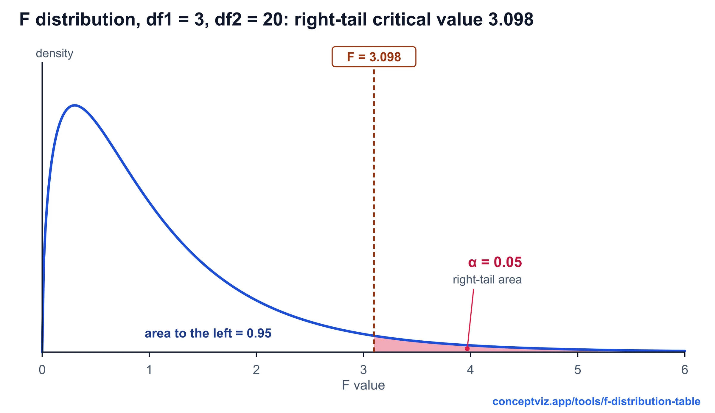
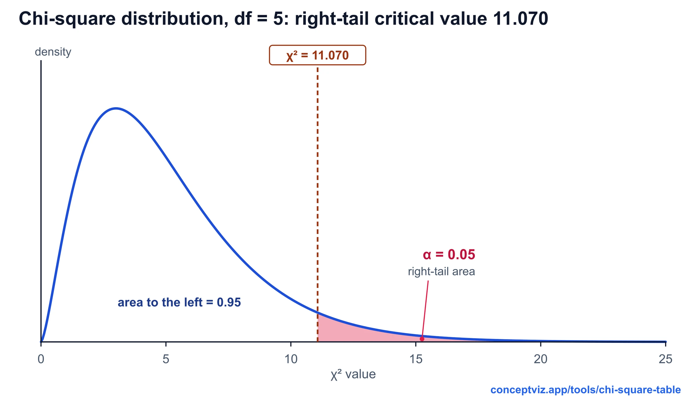
- Then use the calculator above or the quick tables below. For a two-tailed z test at α = 0.05 the value is ±1.960. For a t test with 10 df at the same α it is ±2.228. For chi-square with 5 df and a right-tailed α of 0.05 it is 11.070. For F with 3 and 20 df it is 3.098. As df grows, t approaches z: with infinite df the two-tailed t value is 1.960.
- Confidence level to α: α = 1 − confidence level. For a 90% confidence interval α = 0.10, so the two-tailed z critical value is ±1.645; at 95% it is ±1.960 and at 99% it is ±2.576. The same α with a t distribution gives a larger value for small df.
- In a standard z table, the body holds cumulative areas, so look up 1 − α for a right-tailed test (0.95 for α = 0.05) or 1 − α/2 for a two-tailed test (0.975), then read z from the row and column headers. The area 0.975 sits at z = 1.96.
One-tailed or two-tailed
A two-tailed test looks for a difference in either direction, so α is split between the two tails and each tail holds α/2. A one-tailed test puts all of α in one tail, so the cut-off moves closer to zero: 1.645 instead of 1.960 for z at α = 0.05. Decide the direction from your research question before you see the data, not afterwards. Chi-square and F tests are usually right-tailed because only a large statistic counts as evidence against the null hypothesis. The calculator also returns both cut-offs of a two-tailed chi-square or F test when you need them.
The Pearson r critical values table
- The Pearson r table answers a different question: how large must a sample correlation be before it is unlikely to come from a population with no correlation? The degrees of freedom are n − 2, where n is the number of pairs. Each value is r = t / √(t² + df), with t the critical value of the t distribution at the same df and α. The test assumes a roughly linear relationship and independent pairs, and, for small samples, roughly normal data.
- Take 12 pairs of measurements. Then df = 10. At two-tailed α = 0.05 the table gives 0.576, so a correlation with |r| above 0.576 is significant. At α = 0.01 with 22 pairs (df = 20) the value is 0.537. The same r from a larger sample is easier to call significant, which is why a significant r is not automatically a strong one.
Missing rows and rounding
Printed tables skip some df. For t, F and Pearson r, the cautious habit is to use the next smaller df listed, which gives a slightly larger critical value. Chi-square works the other way: its critical value grows with df, so use the next larger df listed to stay on the safe side, or interpolate between the two rows. The calculator removes the guesswork: type any whole df and it returns the value directly. All values here are rounded to 3 decimals with ordinary rounding, and the calculator also shows more digits. Printed tables can differ in the last digit because of rounding, so check how a textbook rounds and which df it uses.
Frequently Asked Questions
Related Statistics Tools
 Research
P-Value Table
Turn a z, t, chi-square, F or r statistic into a p-value and see how to report it in APA style.
 Research
T Table
T table with one-tailed and two-tailed critical values for df 1 to 120 and infinity, a critical value and p-value calculator, and printable sheets.
 Research
Chi-Square Table
Chi-square table with right-tail critical values for df 1 to 100, a p-value calculator with shaded area and lower-tail columns. Print or download.