Chi-Square Calculator
Run a chi-square test of independence or goodness of fit on a table up to 5x5, see expected counts, residuals, Cramer's V and p-value. Free.
| Observed counts | Total | ||
|---|---|---|---|
| 50 | |||
| 50 | |||
| Total | 45 | 55 | 100 |
Yates continuity correction (2 × 2 only)
Up to 5 × 5. Enter counts, not percentages.
χ² statistic
9.091
Degrees of freedom
1
p-value
0.0026
Cramér's V
0.302
medium effect
φ (phi)
0.302
sign follows row and column order
Fisher exact p
0.0046
two-sided, 2 × 2
p is below 0.05. The counts differ from what independence predicts by more than chance alone would usually produce, so the rows and columns look related.
APA result
χ²(1, N = 100) = 9.09, p = .003, φ = .30
Expected counts
| Improved | Not improved | |
|---|---|---|
| Treatment | 22.5 | 27.5 |
| Control | 22.5 | 27.5 |
Expected = row total × column total ÷ N. Cells under 5 are highlighted.
Standardized residuals
| Improved | Not improved | |
|---|---|---|
| Treatment | +3.02 | -3.02 |
| Control | -3.02 | +3.02 |
(O − E) ÷ √(E × (1 − row share) × (1 − column share)). Blue means more than expected, orange fewer; bold is beyond ±1.96.
Residual heatmap
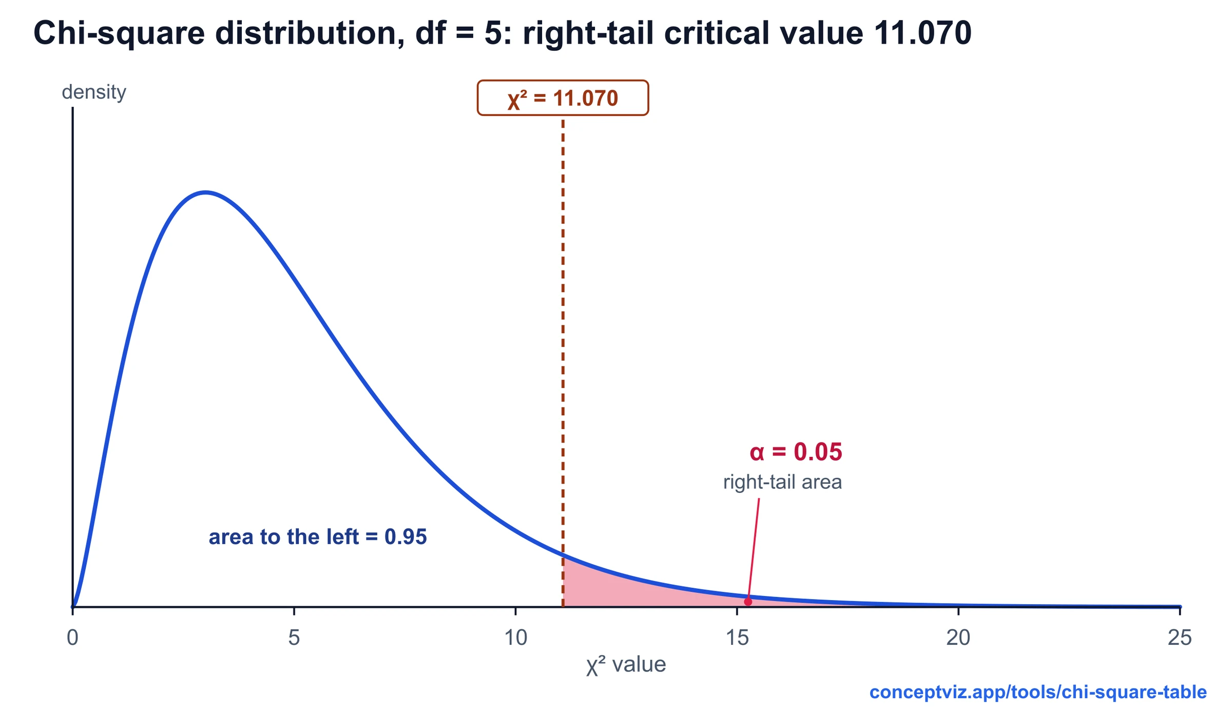
Want the critical value instead of the p-value? Look up df = 1 in the chi-square table.
Free Chi-Square Calculator Charts
Every chart below is drawn from the same code as the calculator above. View and download them free, no sign-up.
Chi-Square Residual Heatmap (2 × 3)
Observed count, expected count and adjusted residual in every cell: χ² = 11.111, df 2, p = 0.0039.
Worked examples
How to calculate
How to choose
To compare your statistic with a cut-off instead of a p-value, use the chi-square table. To compute d, g or eta squared for numeric data, try the effect size calculator, and to turn a grid of values into a color-coded chart, use the heatmap generator. To lay out your counts as a labeled table first, use the two-way table generator.
What a chi-square test tells you
- A chi-square (χ²) test compares counts you observed with the counts you would expect if a simple hypothesis were true. The statistic is the sum of (observed − expected)² ÷ expected over every cell or category. The more the data depart from the hypothesis, the larger χ² gets, and the p-value is the chance of a statistic at least that large when the hypothesis holds. The test works on counts of people, events or items, never on percentages or means.
- This calculator runs both common versions. Use the test of independence when each observation falls into one row and one column of a table, for example treatment group by outcome. Use goodness of fit when one categorical variable has a hypothesis for the share of each category, such as an even split or a 9:3:3:1 ratio.
Independence or goodness of fit?
The test of independence asks whether two categorical variables are related. Expected counts come from the margins: row total × column total ÷ N, and the degrees of freedom are (rows − 1) × (columns − 1). Goodness of fit asks whether one variable follows a stated distribution. Expected counts are the hypothesised share × N, and the degrees of freedom are categories − 1, minus one more for each parameter estimated from the data. Both use the same right-tail p-value; only the way the expected counts and degrees of freedom are found differs.
Assumptions to check first
Each observation must be counted once and be independent of the others, so repeated measures on the same person need a different test. The categories must not overlap. The usual rule of thumb is that expected counts should be about 5 or more, and the calculator warns you when more than 20% of the cells fall below 5. For a 2 × 2 table it then shows Fisher’s exact test, which does not rely on the χ² approximation. A larger table with sparse cells can often be fixed by combining categories that make sense together.
How to read expected counts and residuals
- The χ² statistic only says that something differs. The residuals say where. The standardized residual here is the adjusted one, (O − E) ÷ √(E × (1 − row share) × (1 − column share)), which behaves roughly like a z-score. A value beyond ±1.96 marks a cell that departs from independence at about the 5% level; positive means more observations than expected, negative fewer. In the 2 × 3 example above, the Group A / Low cell has an adjusted residual of 3.33, the largest single share of the χ² of 11.111. For goodness of fit the table shows the simpler Pearson residual (O − E) ÷ √E, where about ±2 is large.
- With many cells, expect an occasional large residual by chance alone, so read the pattern rather than a single cell.
Yates correction, Fisher and effect size
- A significant p-value does not say how strong the link is, so the calculator also reports Cramér's V, which runs from 0 to 1 (φ for a 2 × 2 table), and Cohen's w for goodness of fit. For a 2 × 2 table, Yates' continuity correction subtracts 0.5 from each |O − E| before squaring. It is off by default and available only for 2 × 2 tables. On the table [[10, 20], [30, 40]] it changes χ² from 0.794 to 0.446 and p from 0.3730 to 0.5040; Fisher's exact test gives p = 0.5045. Cramér's V and φ are always computed from the uncorrected χ².
Frequently Asked Questions
Related Statistics Tools
 Research
Chi-Square Table
Chi-square table with right-tail critical values, df 1 to 100, a p-value calculator with shaded area and lower-tail columns. Printable.
 Research
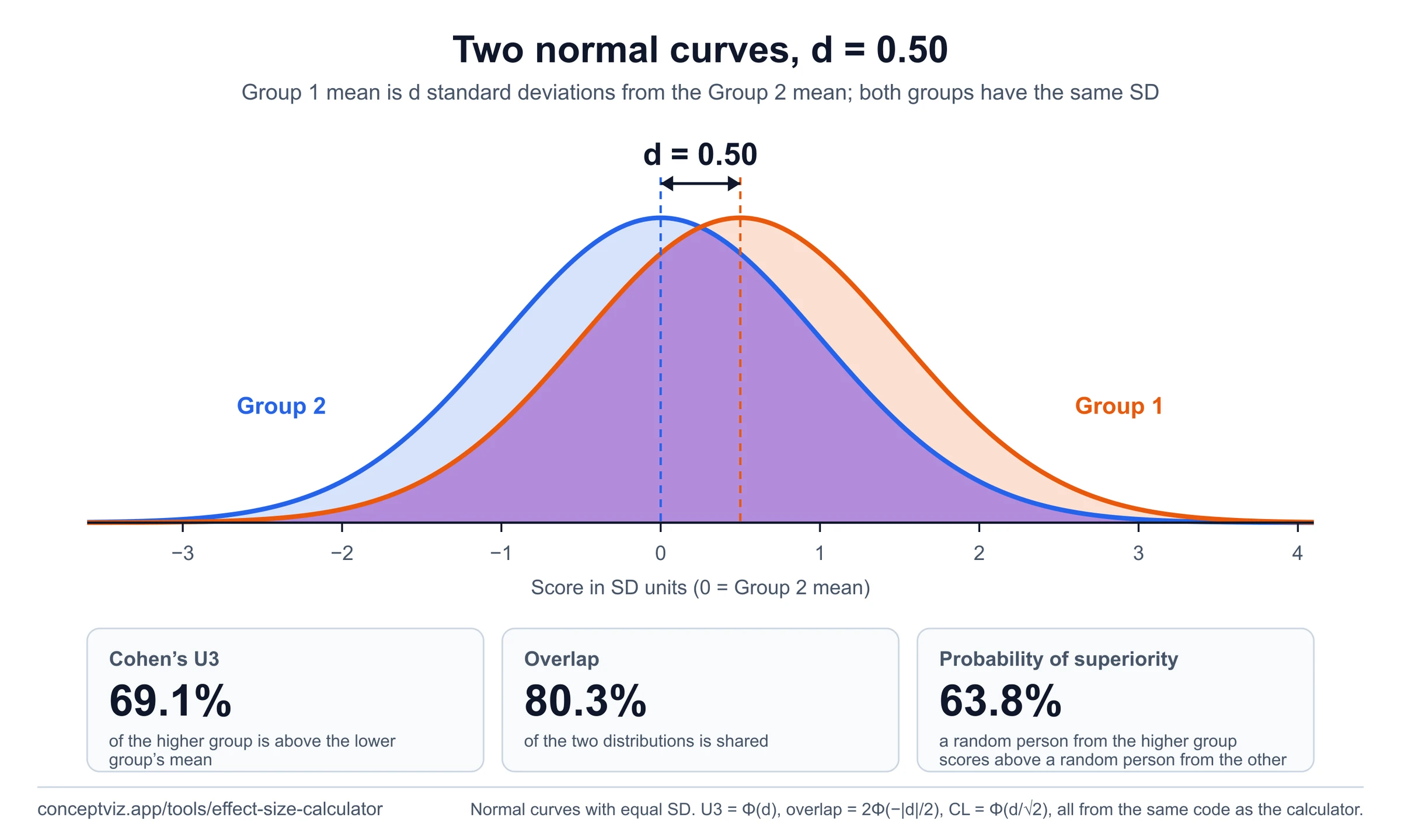
Effect Size Calculator
Compute Cohen’s d, Hedges’ g, eta squared and more from your own summary statistics.
 Research
Two-Way Table Generator
Build a two-way (contingency) table from two categorical variables with row and column totals, then export SVG or PNG.
 Research
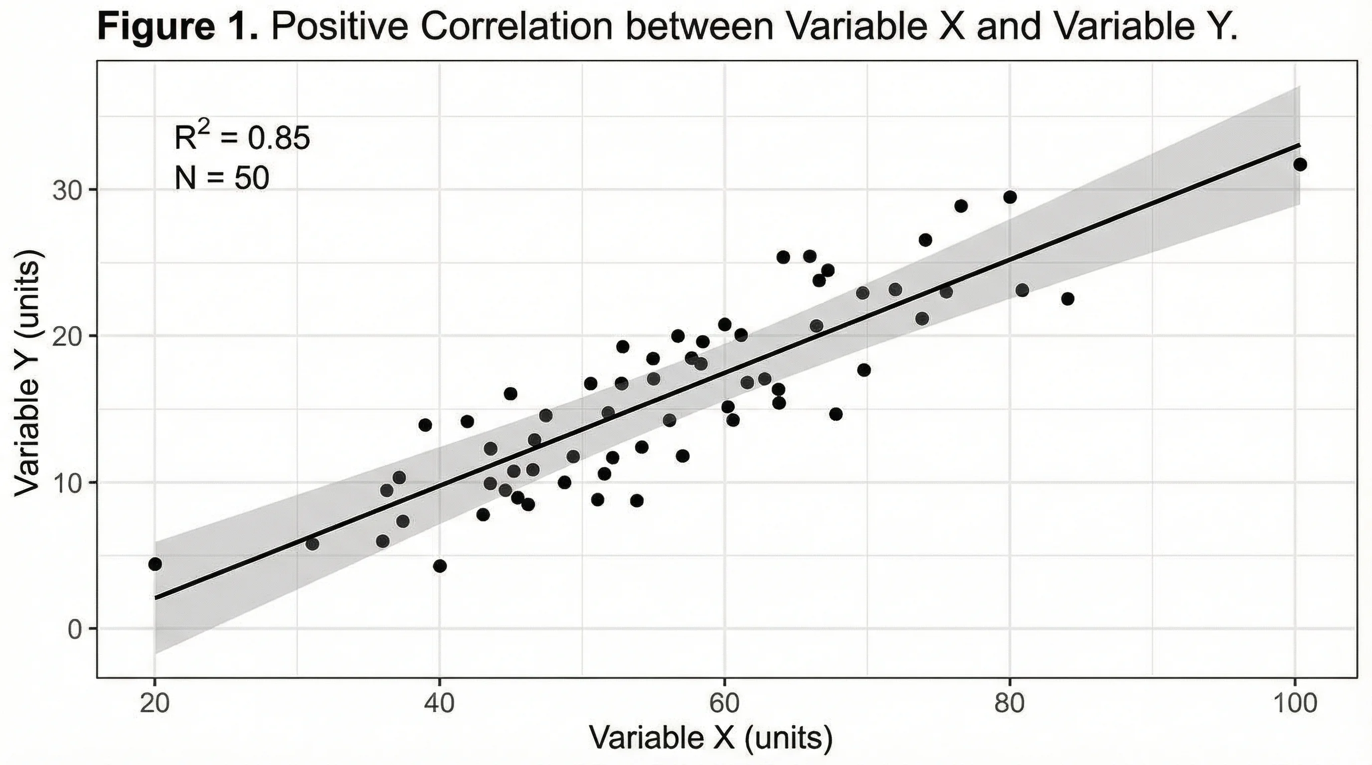
Heatmap Generator
Turn a grid of values into a labeled heatmap with a color scale and export it as SVG or PNG.
 Research
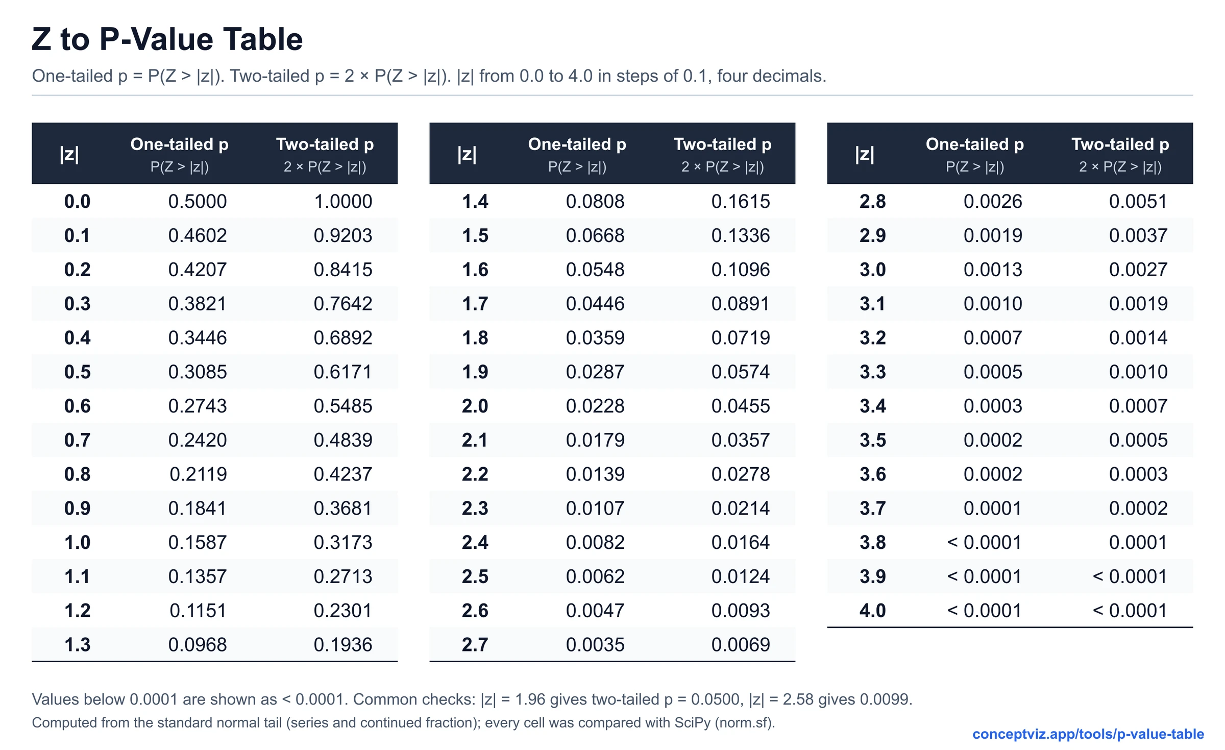
P-Value Table
Turn a test statistic into a p-value for z, t, chi-square and F with a shaded curve.
 Research
Critical Values Table
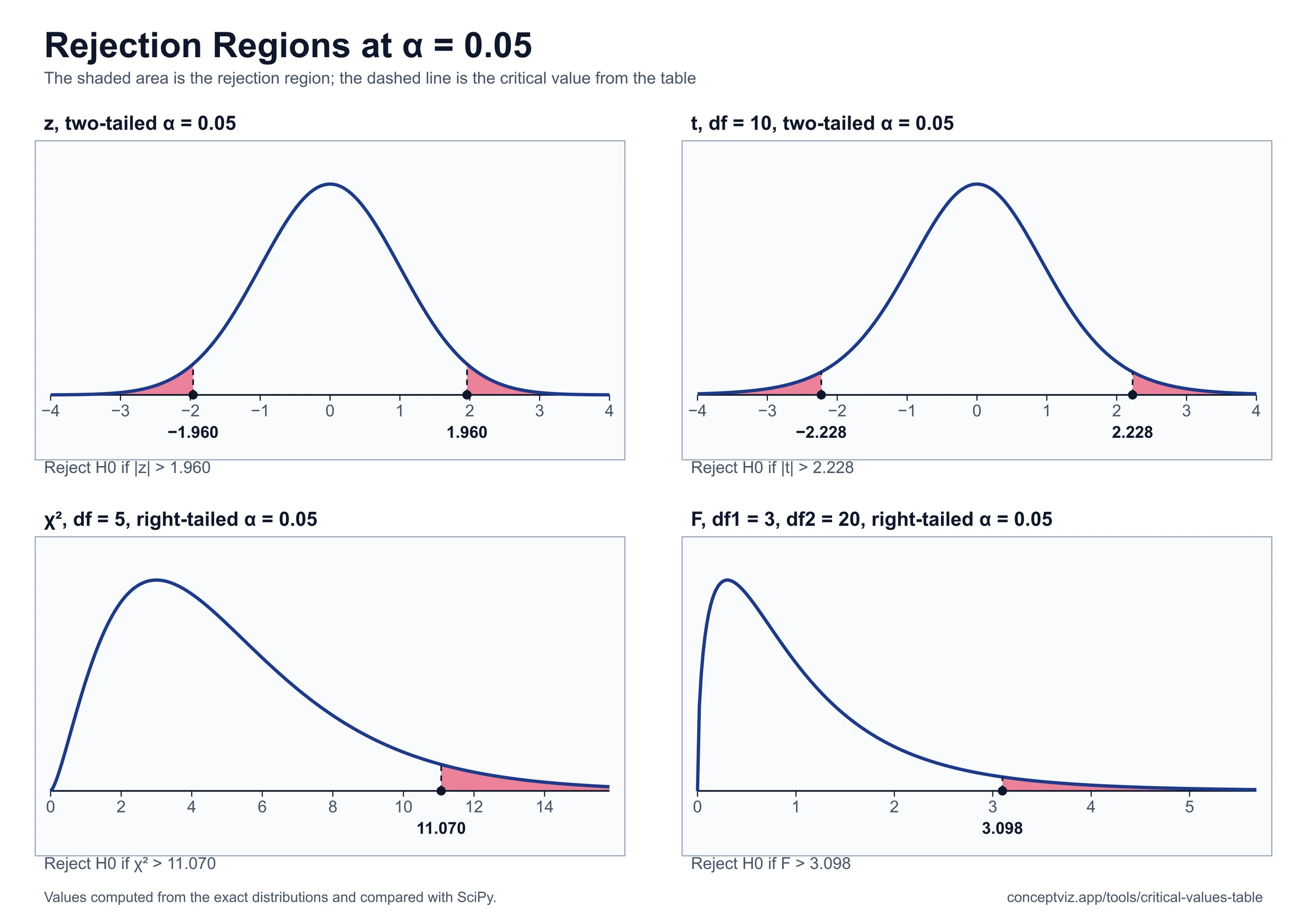
Chi-square, z, t, F and r cut-offs side by side with a critical value calculator.