Nyquist Plot Generator for G(jω)
Free Nyquist plot generator. Enter a transfer function to draw G(jω) on the complex plane, then download SVG.
Enter numerator and denominator coefficients — renders G(jω) on the complex plane as SVG, free
Transfer function
Coefficients in descending powers of s, same as the Bode page. This tool does not run the full Nyquist N = P − Z test.
n=240 · closest approach to (−1, 0) is 1.000 at ω=80.000. Distance is a diagnostic, not a stability verdict.
Nyquist Plot Generator
Free to try ·
Your AI Nyquist-plot illustration will appear here
For a data-accurate plot from a transfer function, use the Precise Plot tab instead
Nyquist Plot Examples
The first four are exact engine renders from transfer functions. The last two are AI illustrations of Illustration mode.
First-order low-pass
Exact engine render — H(s) = 1/(s+1), real vs imaginary of G(jω).
Second-order system
Exact engine render — damped second-order plant.
Type-1 plant
Exact engine render — a pole at the origin sends low-ω points down the imaginary axis.
Integrator
Exact engine render — G(jω) = −j/ω.
AI illustration — polar
AI illustration of Illustration mode — visual mockup, not evaluated from G(s).
AI illustration — teaching
AI illustration of Illustration mode — visual mockup, not a stability proof.
What is a Nyquist plot?
A Nyquist plot is the frequency response of a transfer function drawn on the complex plane: the real part of G(jω) on x, the imaginary part on y, as ω runs from near 0 to a large value. Control engineers use it with the Nyquist stability criterion and the critical point (−1, 0). This page evaluates a continuous-time rational G(s) you type as coefficients. It is not a Bode magnitude/phase pair, and it is not the electrochemical impedance plot of Z′ versus −Z″.
How to enter G(s)
- Use the same coefficient convention as the Bode plot generator: descending powers of s. 1 / (s + 1) is numerator 1 and denominator 1, 1. A type-1 plant 1 / (s(s + 1)(s + 2)) is denominator 1, 3, 2, 0.
- The solid curve is ω > 0. The dashed curve is the conjugate mirror for real coefficients (ω < 0). The red dot is (−1, 0). Distance from the curve to that point is printed as a diagnostic.
- This page does not count encirclements or apply N = P − Z. For a stability argument you still need the open-loop right-half-plane pole count from your notebook.
Nyquist plot versus a Bode plot
Both come from G(jω). A Bode plot splits that number into magnitude (dB) and phase (degrees) versus log frequency. A Nyquist plot keeps the complex number as one polar curve. Use this page for the complex-plane figure; use the Bode plot generator for the two-panel frequency-response figure.
Export
Download a scalable SVG with no watermark and no account required for the precise plot. The AI Illustration tab is only for slides when you do not have a transfer function yet — it will not match your G(s).
Frequently Asked Questions
Related Engineering Tools
 Engineering
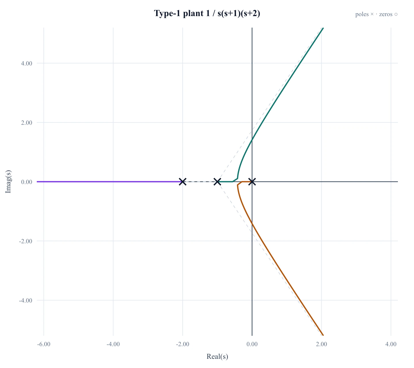
Root Locus Plot Generator
Need closed-loop poles versus gain K in the s-plane? That is a root locus, not a Nyquist plot.
 Engineering
Bode Plot Generator
Need magnitude and phase versus log frequency instead? That is a Bode plot, not a Nyquist plot.
 Engineering
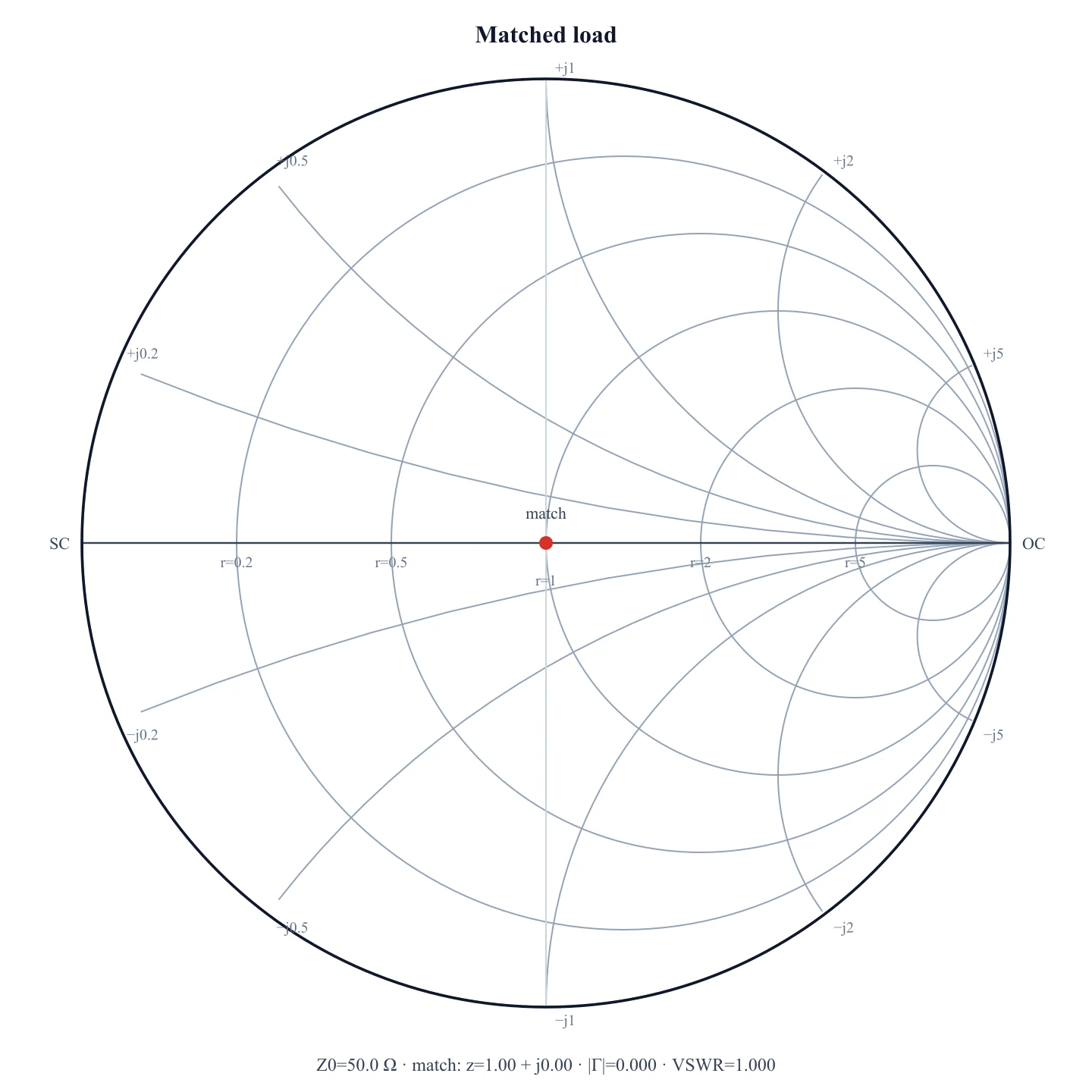
Smith Chart Generator
Need Γ of an RF load on a transmission line? That is a Smith chart, not a Nyquist plot of G(jω).
 Engineering
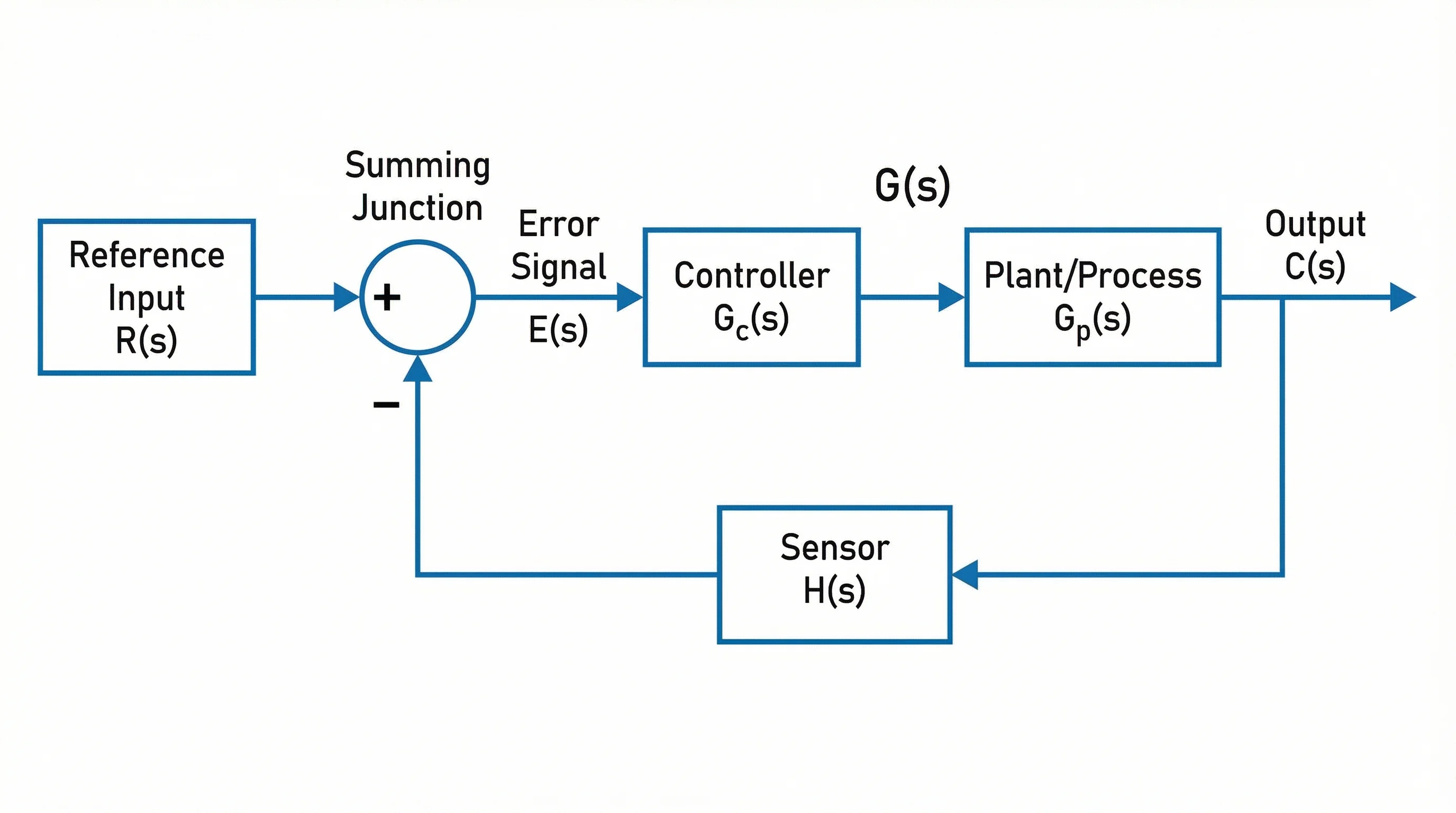
Block Diagram Generator
Sketch the plant, controller, and feedback loop that the transfer function came from.
 Physics
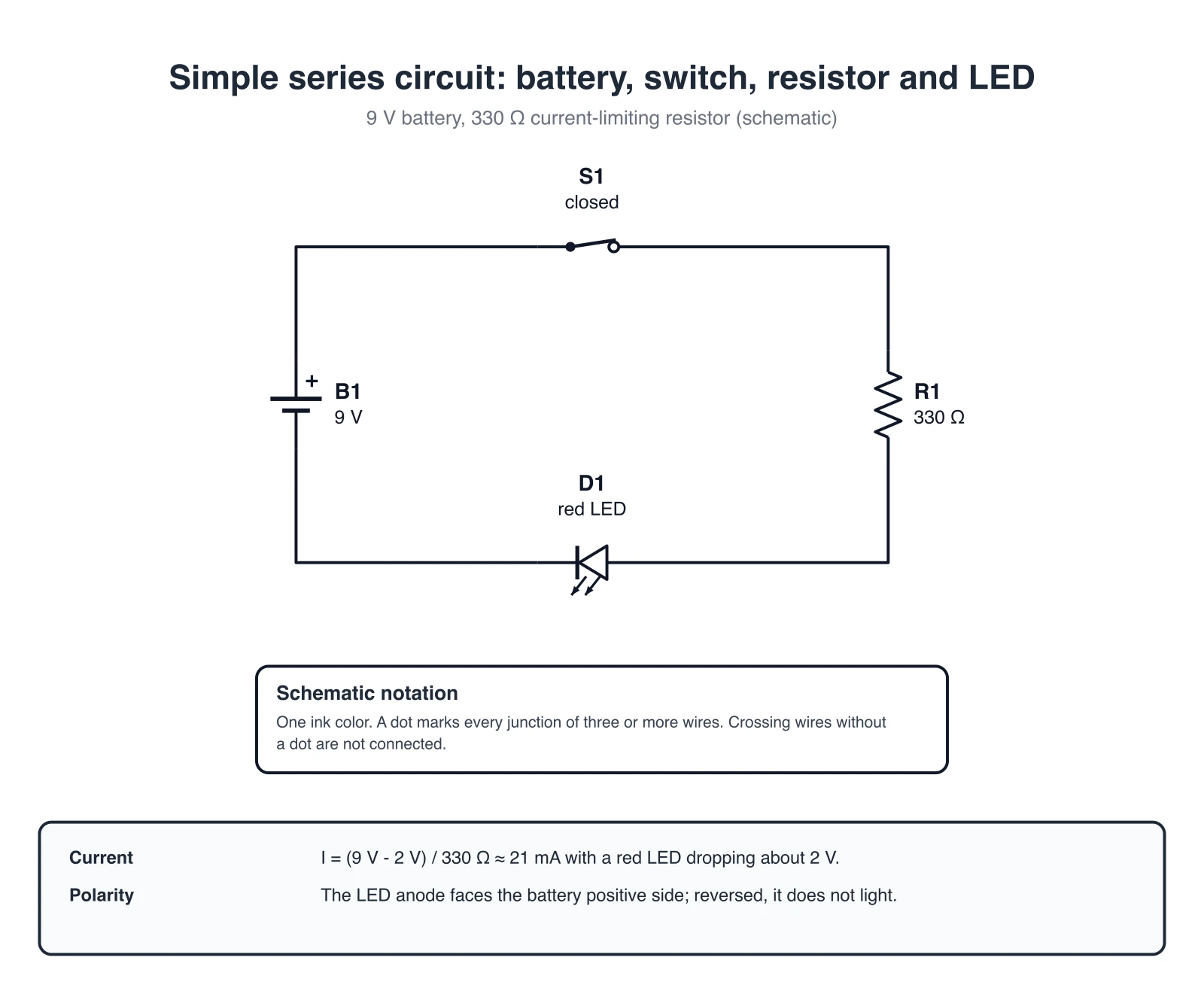
Circuit Diagram Maker
Draw the analog filter or compensator whose G(s) you just plotted.