How do I make a root locus from a transfer function?

Enter numerator and denominator coefficients in descending powers of s, plus an optional gain. The tool sweeps K in 1 + K G(s) = 0 and draws the closed-loop pole paths. Download the SVG for a report or slide.

What does a root locus tell you?

It shows how closed-loop poles move as gain changes: damping, oscillation frequency, and whether branches cross the imaginary axis. This page draws the paths. It does not output a stability certificate.

Is this the same as a Bode or Nyquist plot?

No. Bode is magnitude and phase versus frequency. Nyquist is Re(G(jω)) versus Im(G(jω)). A root locus is closed-loop poles versus gain K in the s-plane. Same G(s), different figure.

Does this run MATLAB rlocus or design a compensator?

No. It is a teaching plot of 1 + K G(s) = 0. It does not call MATLAB, does not add lead/lag zeros, and does not pick K for a target ζ.

Why are poles × and zeros ○?

That is the usual Evans symbol language. Open-loop poles start the branches. Finite zeros attract branches as K grows. Branches that have no finite zero go to infinity along the dashed asymptotes.

Is the root locus plot generator free?

The precise, coefficient-driven plot is free to use and free to download as SVG, with no sign-up. Sign in only if you want AI illustrations or other ConceptViz generation tools.

Control Systems Tool

Root Locus Plot Generator Evans s-plane

Free root locus generator. Enter G(s) coefficients to draw Evans closed-loop pole paths, then download SVG.

Numerator / denominator coefficientsClosed-loop poles versus KPoles × and zeros ○Download a watermark-free SVG — free

Enter numerator and denominator coefficients — renders Evans closed-loop pole paths as SVG, free

Transfer function

Coefficients in descending powers of s, same as the Bode and Nyquist pages. This tool sweeps K in 1 + K G(s) = 0. It does not design a compensator.

NumeratorDenominatorGain in G(s)

Title

Asymptotesζ ≈ 0.707 damping rays

n=3 open-loop poles · m=0 finite zeros. Paths are 1 + K G(s) = 0 as K increases. Not MATLAB rlocus, and not a stability certificate.

Root Locus Examples

The first four are exact engine renders from transfer functions. The last two are AI illustrations of Illustration mode.

View:

Type-1 plant

Exact engine render — textbook three-pole plant, poles as ×.

root-locustype-1

Complex poles

Exact engine render — open-loop poles already off the real axis.

root-locussecond-order

Finite zero

Exact engine render — zeros stay put as ○ while poles move.

root-locuszero

First-order pole

Exact engine render — a single real branch as K grows.

root-locusfirst-order

AI illustration — Evans

AI illustration of Illustration mode — visual mockup, not computed from G(s).

aiillustration

AI illustration — teaching

AI illustration of Illustration mode — visual mockup, not a compensator design.

aiillustrationteaching

What is a root locus?

A root locus (Evans plot) shows where the closed-loop poles of 1 + K G(s) = 0 travel in the s-plane as the gain K goes from 0 to a large value. Open-loop poles start as ×. Finite zeros are ○ and do not move with K. This page evaluates a continuous-time rational G(s) you type as coefficients. It is not a Bode magnitude/phase pair, and it is not a Nyquist plot of G(jω).

How to enter G(s)

Use the same coefficient convention as the Bode and Nyquist generators: descending powers of s. The textbook plant 1 / (s(s + 1)(s + 2)) is numerator 1 and denominator 1, 3, 2, 0.
The engine solves den(s) + K · gain · num(s) = 0 on a log-spaced K grid, then tracks branches. Dashed lines are the large-K asymptotes. Optional rays mark ζ ≈ 0.707.
This page does not run MATLAB rlocus, does not place a lead/lag compensator, and does not print a stable/unstable verdict. Axes use equal real and imaginary scales so the silhouette matches a textbook s-plane.

Root locus versus Bode and Nyquist

All three start from the same G(s). Bode splits G(jω) into magnitude and phase versus log frequency. Nyquist keeps G(jω) as one polar curve. Root locus never evaluates jω; it plots closed-loop poles versus K. Use this page for the Evans figure.

Export

Download a scalable SVG with no watermark and no account required for the precise plot. The AI Illustration tab is only for slides when you do not have a transfer function yet — it will not match your G(s).

Frequently Asked Questions

Related Engineering Tools

Engineering

Nyquist Plot Generator

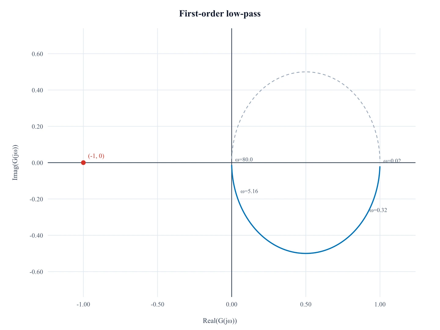
Need Re(G(jω)) versus Im(G(jω)) instead? That is a Nyquist plot, not an Evans locus.

Try it free

Engineering

Bode Plot Generator

Need magnitude and phase versus log frequency? That is a Bode plot, not a root locus.

Try it free

Engineering

Block Diagram Generator

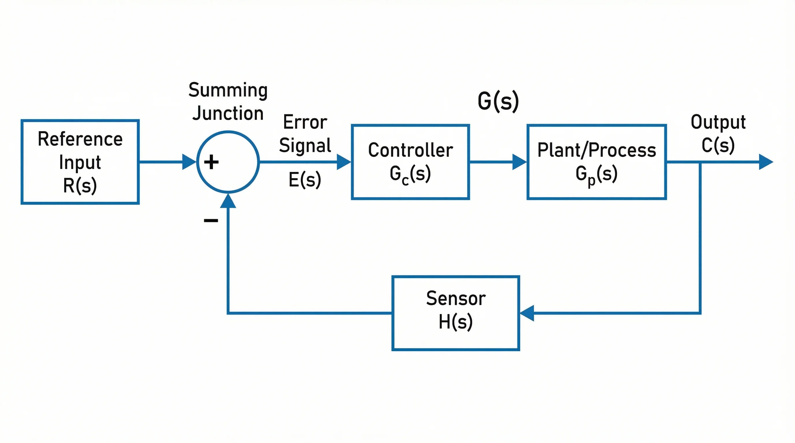
Sketch the plant, controller, and feedback loop that the transfer function came from.

Try it free

View All Free Tools

What is a root locus?

How to enter G(s)

Use the same coefficient convention as the Bode and Nyquist generators: descending powers of s. The textbook plant 1 / (s(s + 1)(s + 2)) is numerator 1 and denominator 1, 3, 2, 0.

The engine solves den(s) + K · gain · num(s) = 0 on a log-spaced K grid, then tracks branches. Dashed lines are the large-K asymptotes. Optional rays mark ζ ≈ 0.707.

This page does not run MATLAB rlocus, does not place a lead/lag compensator, and does not print a stable/unstable verdict. Axes use equal real and imaginary scales so the silhouette matches a textbook s-plane.