Calibration Curve Generator for standard curves
Free calibration curve generator. Paste standard concentrations and signals to fit a line, read unknowns, and download SVG.
Paste standard concentrations and signals — fits a line, reads unknowns, downloads SVG, free
Standards
Paste concentration, then signal. This is an analytical standard curve. It is not a titration, a residual plot, or ML probability calibration.
6 standards parsed
n=6 · y = 0.021 + 0.093x · R²=0.9999 · unknowns: 0.45→4.622, 0.7→7.319, 0.88→9.260. This page does not report LOD/LOQ or weighted least squares.
Calibration Curve Generator
Free to try ·
Your AI calibration-curve illustration will appear here
For a data-accurate plot from standards, use the Precise Plot tab instead
Calibration Curve Examples
The first four are exact engine renders from tables. The last two are AI illustrations of Illustration mode.
Beer’s law
Exact engine render — pasted standards, linear fit, unknown signals marked.
HPLC peak area
Exact engine render — peak area versus concentration.
Fluorescence
Exact engine render — intensity versus nM standards.
Quadratic range
Exact engine render — quadratic fit through six standards.
AI illustration — Beer’s law
AI illustration of Illustration mode — visual mockup, not plotted from standards.
AI illustration — teaching
AI illustration of Illustration mode — visual mockup, not a fitted assay.
What is a calibration curve?
An analytical calibration curve — also called a standard curve — plots instrument signal against known concentrations, then fits a line (or a shallow quadratic) so you can read unknown samples. Spectrophotometry uses absorbance; chromatography uses peak area; fluorescence uses intensity. This page draws that figure from standards you already measured. It does not run weighted least squares, report LOD/LOQ, or draw a machine-learning reliability diagram of predicted probabilities.
How to read the fit and the unknowns
- Paste concentration in the first column and signal in the second. Linear mode is ordinary least squares: y = a + bx. Quadratic mode adds a cx² term when the assay bends at high concentration. Unknown signals, one per line, are inverted through the same equation and marked on the plot.
- A residual plot is the leftover y − ŷ against fitted values — use it to check the fit, not to report concentration. A titration curve is pH versus titrant volume. A solubility curve is grams of salt versus temperature.
Calibration curve versus a residual plot or titration
Use this page when you have standards and need the working curve plus inverse predictions. Use the residual plot generator to inspect whether a straight line is honest. Use the titration curve generator for acid–base pH jumps. Standard curve is a synonym and is absorbed here, not a second page.
Export
Download a scalable SVG with no watermark and no account required for the precise plot. The AI Illustration tab is only for slides when you do not have standards yet — it will not match your assay.
Frequently Asked Questions
Related Research Tools
 Research
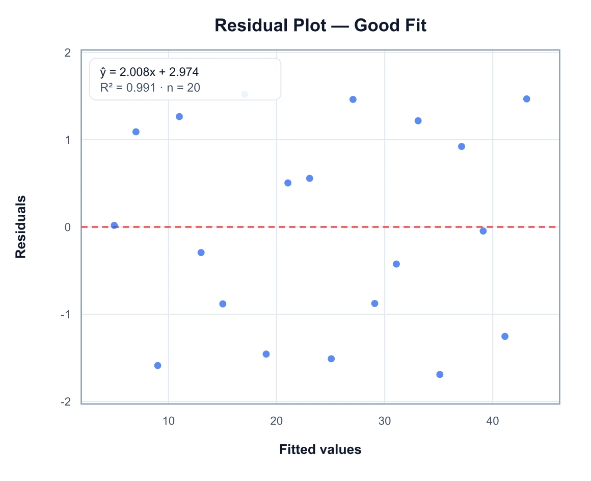
Residual Plot Generator
Check whether the linear fit is honest: residuals against fitted values, not concentration.
 Chemistry
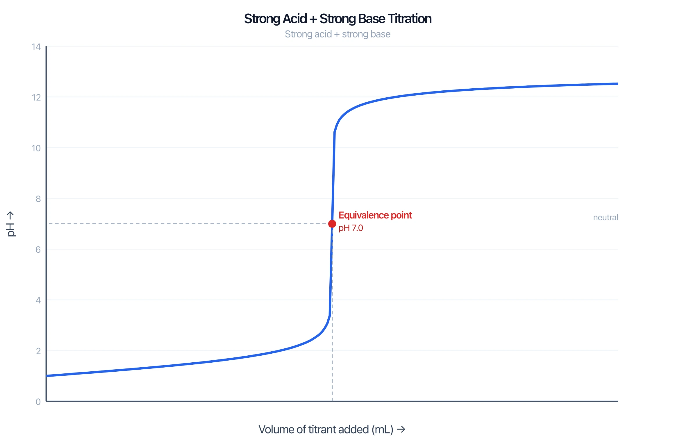
Titration Curve Generator
Need pH versus titrant volume? That is a titration curve, not a standard curve.
 Chemistry
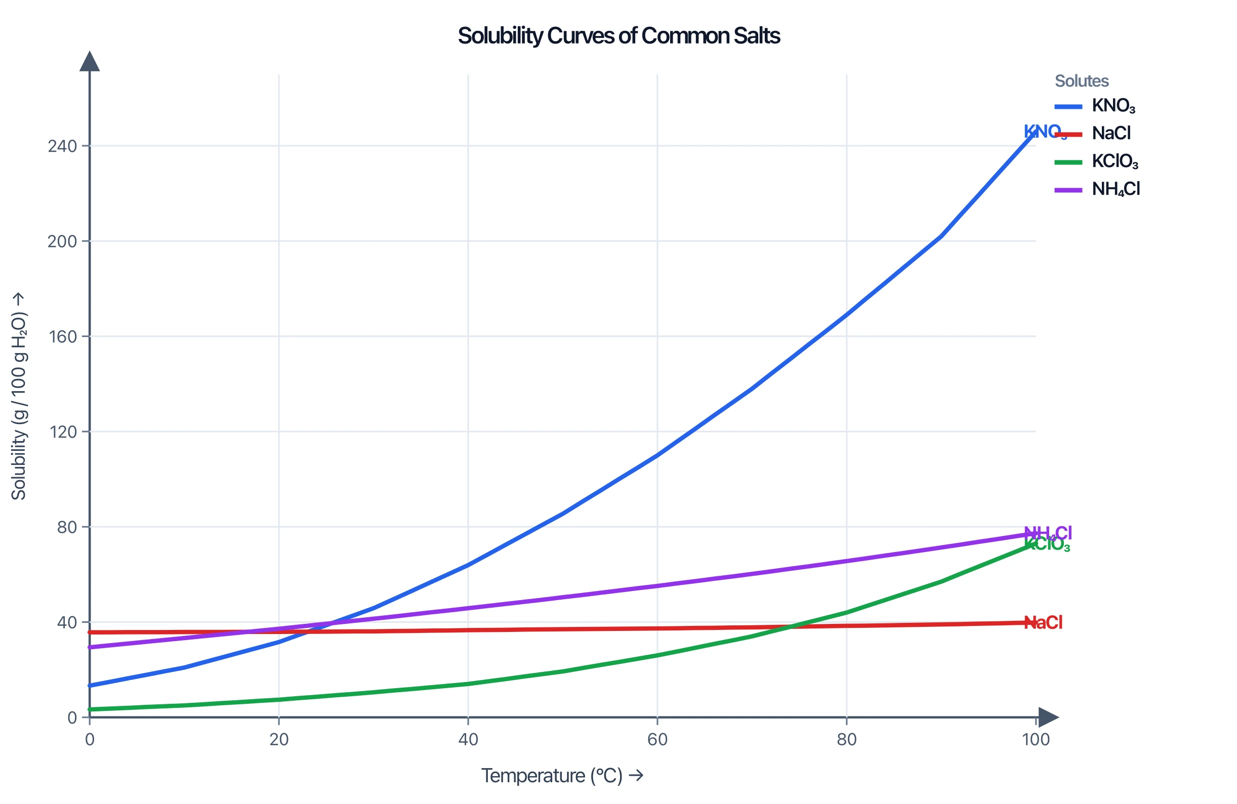
Solubility Curve
Solubility versus temperature is a different lab chart — grams of salt, not assay signal.
 Research
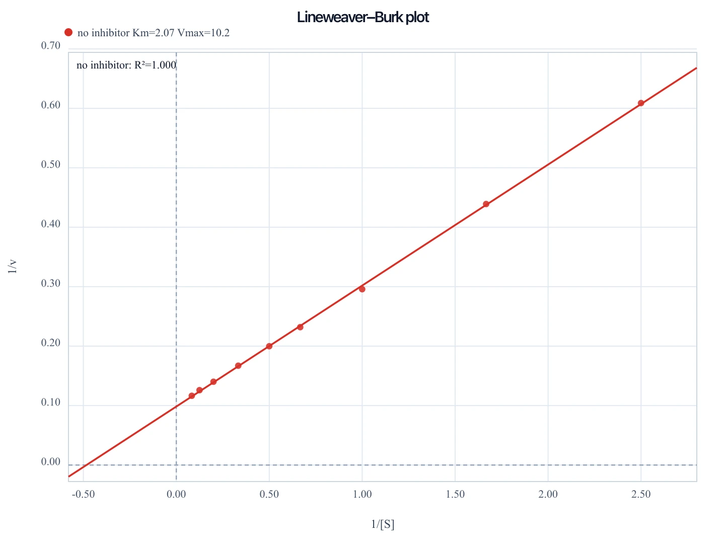
Lineweaver–Burk Plot Generator
Enzyme double-reciprocal plots are kinetics, not a spectrophotometer standard curve.
 Education
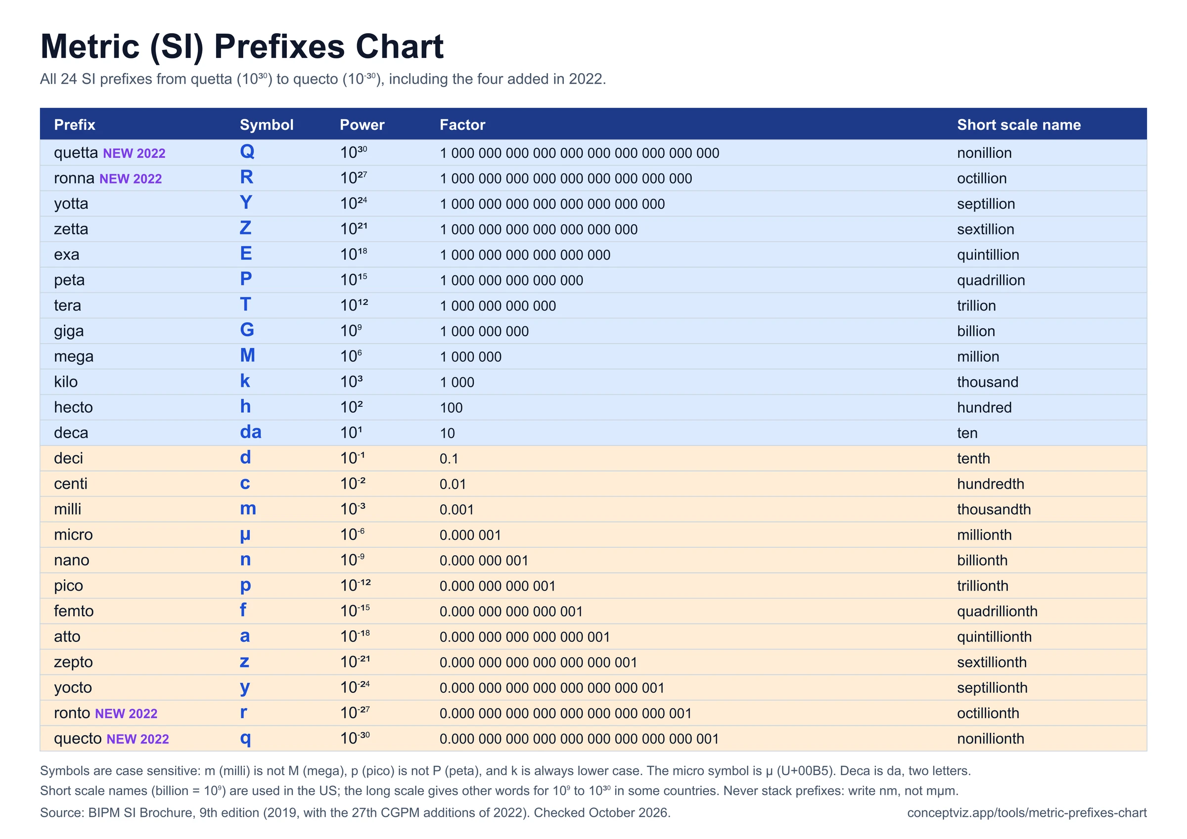
Metric Prefixes Chart
Convert between mg, µg and ng with an exact SI prefix converter and a printable prefix table.