Refrigeration Cycle Diagram Generator with P-h Diagram
Set the evaporating and condensing temperatures, or type your own state points. The schematic, the pressure-enthalpy diagram on real R-134a saturation data and the COP update as you type, ready to export as SVG, PNG or CSV.
R-134a cycle
Set the operating temperatures, or enter your own state points. The diagram, the P-h chart and the COP update as you type.
Assumes saturated vapor into the compressor, saturated liquid out of the condenser, isenthalpic expansion and no pressure drops. At 100% efficiency compression is isentropic.
Scroll the diagram sideways, or use View image for a full-size look.
| State | Condition | T (°C) | P (bar) | h (kJ/kg) |
|---|---|---|---|---|
| 1 | Saturated vapor | −10.0 | 2.006 | 392.66 |
| 2 | Superheated vapor | 46.3 | 10.166 | 426.45 |
| 3 | Saturated liquid | 40.0 | 10.166 | 256.41 |
| 4 | Liquid-vapor, x = 0.34 | −10.0 | 2.006 | 256.41 |
- q_L = h1 − h4 =
- 136.25 kJ/kg
- w = h2 − h1 =
- 33.79 kJ/kg
- q_H = h2 − h3 =
- 170.04 kJ/kg
- COP (heating) = q_H / w =
- 5.03
- Carnot COP at the same temperatures = T_e / (T_c − T_e) =
- 5.26
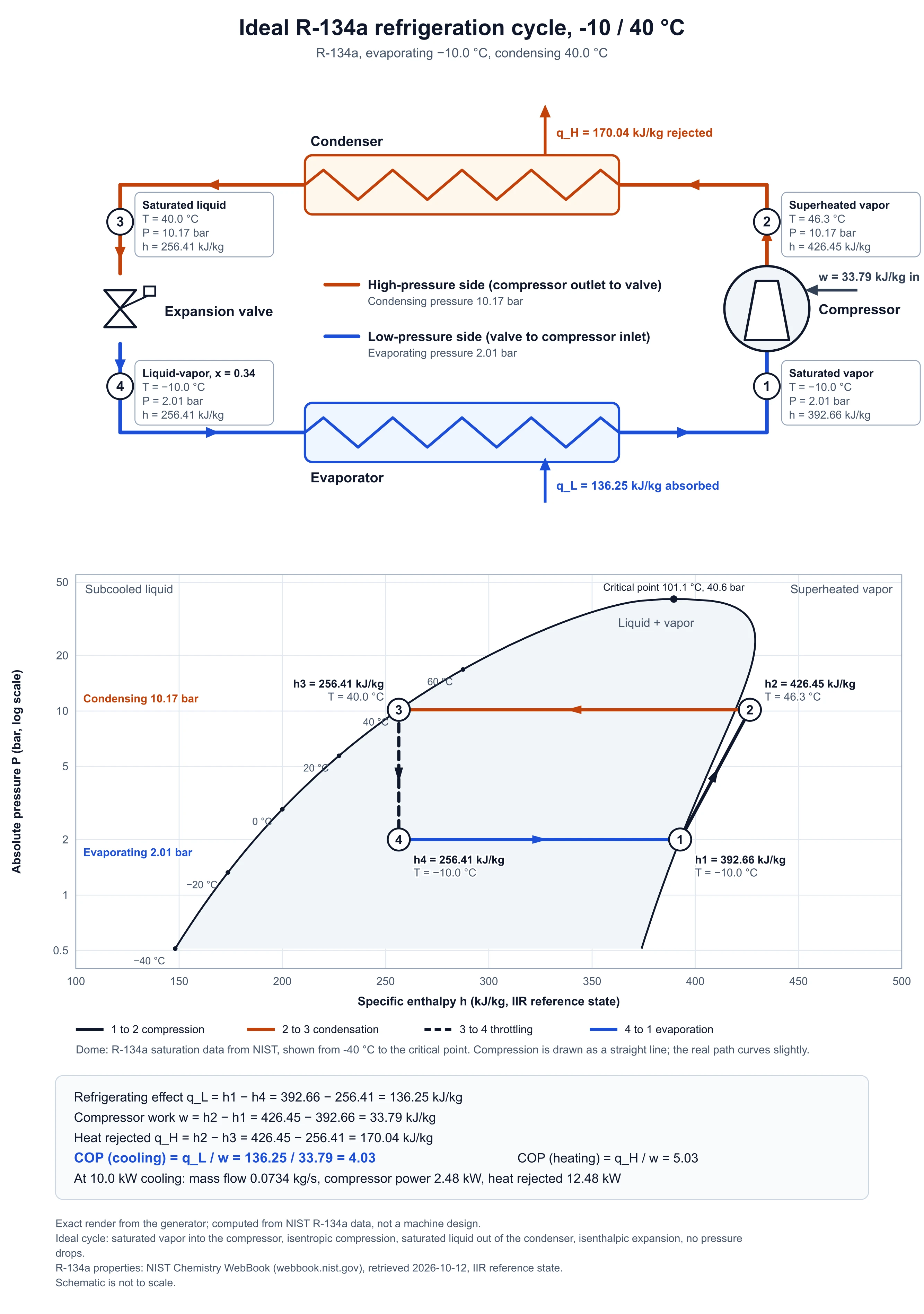
COP = q_L / w = 136.25 / 33.79 = 4.03
What is the refrigeration cycle?
The vapor-compression refrigeration cycle moves heat from a cold space to a warmer one using a refrigerant that is repeatedly evaporated and condensed. Four parts do the work: a compressor, a condenser, an expansion valve and an evaporator. Numbering the refrigerant states 1 to 4 around the loop turns the figure into a calculation: every heat and work quantity is a difference between two enthalpies.
The generator draws that loop as a schematic and, below it, as a pressure-enthalpy (P-h) diagram, the chart engineers use because the evaporator and condenser become horizontal lines and the throttling step a vertical one. The dome is drawn from tabulated R-134a saturation data, so the cycle sits where it really would for the temperatures you choose. For equipment and duct layouts rather than the cycle itself, use the HVAC diagram generator.
The four stages, state by state
- 1
Compression, 1 to 2
Low-pressure vapor from the evaporator is compressed to the condensing pressure. Its pressure, temperature and enthalpy rise, and the work input is w = h2 − h1. An ideal compressor is isentropic; a real one needs more work, which the efficiency field models.
- 2
Condensation, 2 to 3
The hot vapor gives up heat to the outside air or water. It cools to saturated vapor, condenses at constant pressure and leaves as saturated or slightly subcooled liquid. The heat rejected is q_H = h2 − h3.
- 3
Expansion, 3 to 4
The expansion valve (or capillary tube) drops the pressure to the evaporator level. No heat or work is exchanged, so the enthalpy does not change: h4 = h3. Part of the liquid flashes to vapor, which is why state 4 is a liquid-vapor mixture.
- 4
Evaporation, 4 to 1
The cold mixture absorbs heat from the space being cooled and boils at constant pressure. The refrigerating effect is q_L = h1 − h4. An ideal cycle ends this step as saturated vapor.
How to calculate COP, with a worked example
Coefficient of performance for cooling is the useful cooling divided by the work you pay for: COP = q_L / w, with q_L = h1 − h4 and w = h2 − h1 (kJ/kg of refrigerant). The heat rejected is q_H = h2 − h3, and an energy balance gives q_H = q_L + w.
Take an ideal R-134a cycle evaporating at −10 °C (2.006 bar) and condensing at 40 °C (10.166 bar). The NIST table gives saturated vapor at −10 °C h1 = 392.66 kJ/kg and saturated liquid at 40 °C h3 = 256.41 kJ/kg, so h4 = 256.41. Isentropic compression of state 1 to 10.166 bar ends at h2 = 426.45 kJ/kg (46.3 °C). Then:
- q_L = 392.66 − 256.41 = 136.25 kJ/kg
- w = 426.45 − 392.66 = 33.79 kJ/kg
- q_H = 426.45 − 256.41 = 170.04 kJ/kg = 136.25 + 33.79
- COP = 136.25 / 33.79 = 4.03; heating COP = 170.04 / 33.79 = 5.03
The Carnot limit between the same temperatures is T_e / (T_c − T_e) = 263.15 / 50 = 5.26, so the ideal vapor-compression cycle reaches about 77% of it. Enter a cooling capacity in the tool to get the refrigerant mass flow and compressor power: for 10 kW, 10 / 136.25 = 0.0734 kg/s and 0.0734 × 33.79 = 2.48 kW.
How to read a P-h diagram
Enthalpy runs left to right and absolute pressure runs up, usually on a log scale so low and high pressures both fit. Inside the dome the refrigerant is a liquid-vapor mixture; left of it is liquid, right of it is vapor. The cycle is a rectangle with a slanted top-right corner: the bottom line (4 to 1) is the evaporator, the top line (2 to 3) is the condenser, the vertical line (3 to 4) is the expansion valve, and the slanted line (1 to 2) is the compressor. Because energy is read off the horizontal axis, q_L is the width of the bottom line, w is the horizontal run of the slanted one, and a longer compression line at the same q_L means a lower COP.
R-134a saturation table (every 5 °C)
The values behind the dome, from the NIST Chemistry WebBook fluid properties for R-134a, retrieved 2026-10-12. IIR reference state: h = 200 kJ/kg for saturated liquid at 0 °C. Pressures are absolute; hf is saturated liquid and hg saturated vapor.
| T (°C) | P (bar abs.) | hf (kJ/kg) | hg (kJ/kg) |
|---|---|---|---|
| -40 | 0.512 | 148.14 | 374.00 |
| -35 | 0.661 | 154.44 | 377.17 |
| -30 | 0.844 | 160.79 | 380.32 |
| -25 | 1.064 | 167.19 | 383.45 |
| -20 | 1.327 | 173.64 | 386.55 |
| -15 | 1.639 | 180.14 | 389.63 |
| -10 | 2.006 | 186.70 | 392.66 |
| -5 | 2.433 | 193.32 | 395.66 |
| 0 | 2.928 | 200.00 | 398.60 |
| 5 | 3.497 | 206.75 | 401.49 |
| 10 | 4.146 | 213.58 | 404.32 |
| 15 | 4.884 | 220.48 | 407.07 |
| 20 | 5.717 | 227.47 | 409.75 |
| 25 | 6.654 | 234.55 | 412.33 |
| 30 | 7.702 | 241.72 | 414.82 |
| 35 | 8.870 | 249.01 | 417.19 |
| 40 | 10.166 | 256.41 | 419.43 |
| 45 | 11.599 | 263.94 | 421.52 |
| 50 | 13.179 | 271.62 | 423.44 |
| 55 | 14.915 | 279.47 | 425.15 |
| 60 | 16.818 | 287.50 | 426.63 |
| 65 | 18.898 | 295.76 | 427.82 |
| 70 | 21.168 | 304.28 | 428.65 |
| 75 | 23.641 | 313.13 | 429.03 |
| 80 | 26.332 | 322.39 | 428.81 |
Source: NIST Chemistry WebBook, R-134a. The tool uses the full 1 K table.
Superheat and subcooling on the diagram
Superheat is how far the vapor leaving the evaporator is above its saturation temperature at that pressure. It moves state 1 to the right of the dome and keeps liquid out of the compressor. Subcooling is how far the liquid leaving the condenser is below its saturation temperature. It moves state 3 to the left of the liquid line, which also moves state 4 left, because h4 = h3. Both need a pressure converted to a saturation temperature, which is what the table above is for.
A quick estimate with the numbers from the worked example: subcool the 40 °C condenser outlet by 5 K, so the liquid is at 35 °C. Taking its enthalpy as that of saturated liquid at 35 °C (a common approximation, good to a fraction of a percent here), h3 = 249.01 kJ/kg. The refrigerating effect becomes 392.66 − 249.01 = 143.65 kJ/kg, up from 136.25, while the compressor work is unchanged, so COP rises from 4.03 to 4.25. Enter those values in the enthalpy mode to see the shifted states. The temperature mode itself draws the ideal cycle without superheat or subcooling.
Ideal cycle versus a real system
The temperature mode draws the textbook cycle: saturated vapor enters the compressor, saturated liquid leaves the condenser, the valve is isenthalpic and there are no pressure drops. Real systems add superheat at the evaporator outlet, subcooling at the condenser outlet, line losses and a compressor below 100% isentropic efficiency, and they draw their evaporating and condensing temperatures from the heat exchangers and the air or water temperatures. Use the efficiency field for a first look at the penalty, and the enthalpy mode when you have measured or tabulated states.
Common mistakes
- Mixing enthalpy references. Tables and software use different zero points, so an h from one source cannot be subtracted from an h in another. This page uses the IIR reference (200 kJ/kg for saturated liquid at 0 °C); differences between h values are what matter, and they only work within one table.
- Using gauge pressure on the P-h diagram. The axis is absolute pressure. Add about 1.01 bar to a gauge reading before you type it into the manual mode.
- Treating the ideal COP as a machine rating. The ideal cycle has no pressure drops, no superheat or subcooling and a perfect compressor. Measured COP is lower, and the efficiency field only shows the direction.
- Putting state 4 on the saturated liquid line. After the valve the refrigerant is a mixture, so state 4 sits inside the dome at the same enthalpy as state 3.
- Reading the isentropic line as straight. On a log-pressure chart the true compression path curves slightly; this tool draws a straight line between 1 and 2.
Using it responsibly
The tool is for teaching, homework, reports and quick estimates. It covers one refrigerant and one simple cycle, and it does not size equipment or replace manufacturer data and refrigerant handling rules. For equipment drawings, see the HVAC diagram generator or the schematic maker, and see how to make an HVAC diagram for the system-level figure.
Refrigeration Cycle Examples
Exact exports from the generator above, computed from NIST R-134a data
Ideal R-134a Cycle: -10 °C Evaporating, 40 °C Condensing
Exact render: saturated vapor into the compressor, isentropic compression, saturated liquid out of the condenser. COP = 136.25 / 33.79 = 4.03.
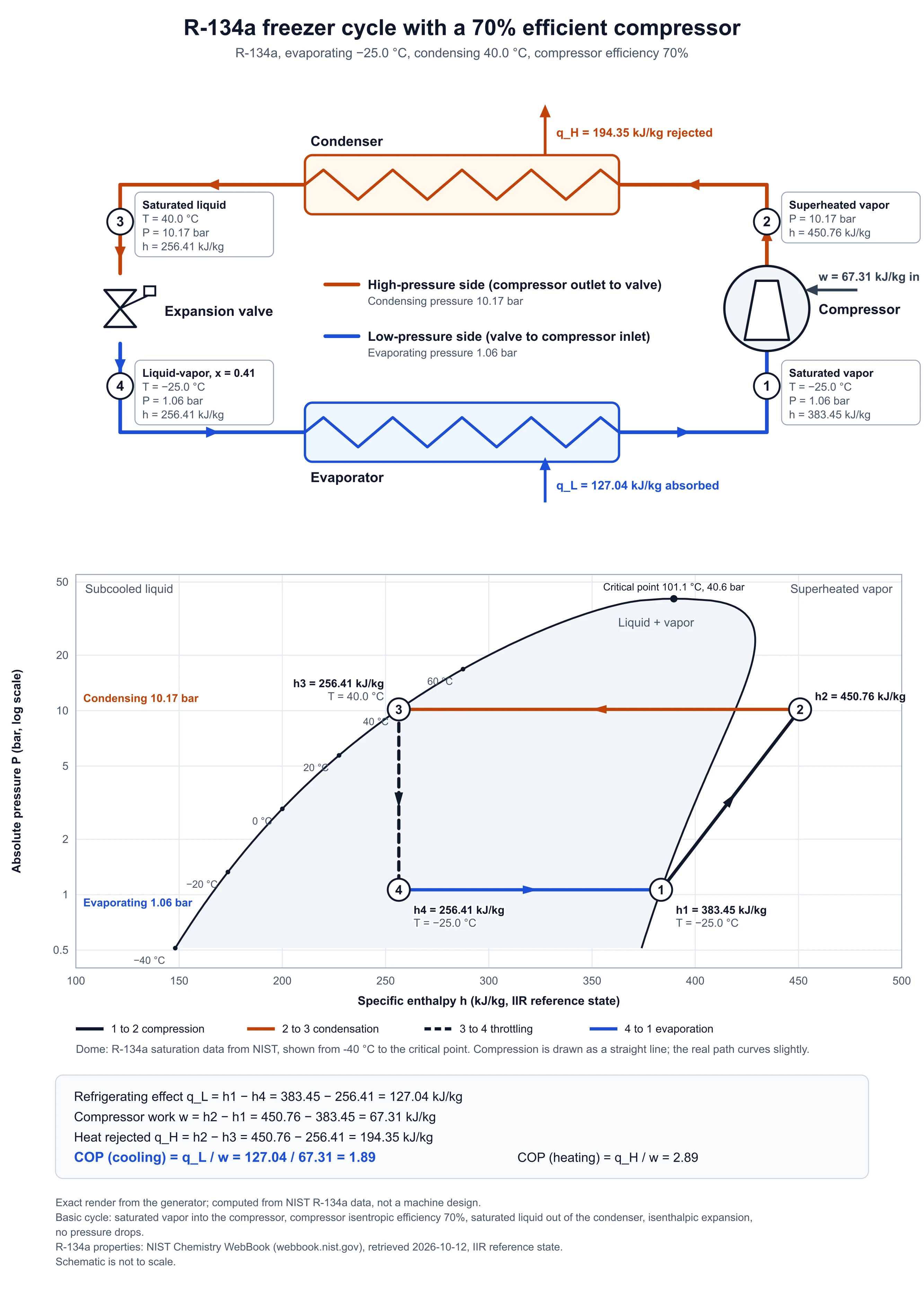
R-134a Freezer Cycle with a 70% Efficient Compressor
Exact render: the same condenser temperature at a colder evaporator and a 70% efficient compressor. COP = 127.04 / 67.31 = 1.89.
Frequently Asked Questions
Related Engineering Tools
 Engineering
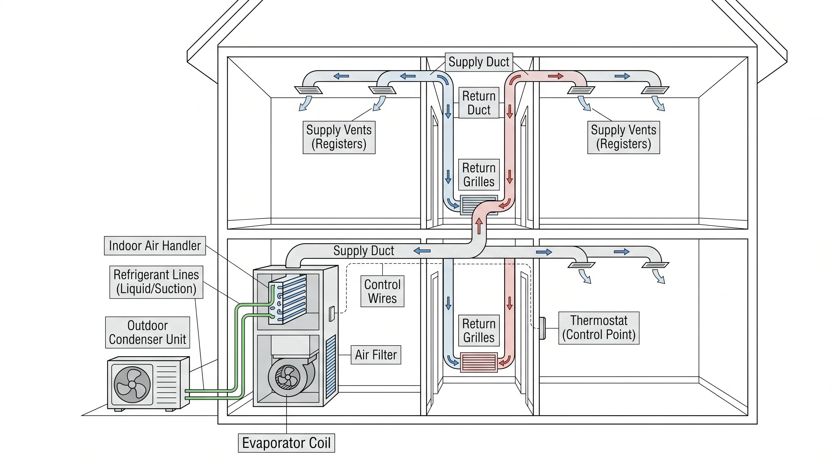
HVAC Diagram Generator
Draw the whole system, ducts and equipment layouts, when you need a plant figure rather than the thermodynamic cycle.
 Science
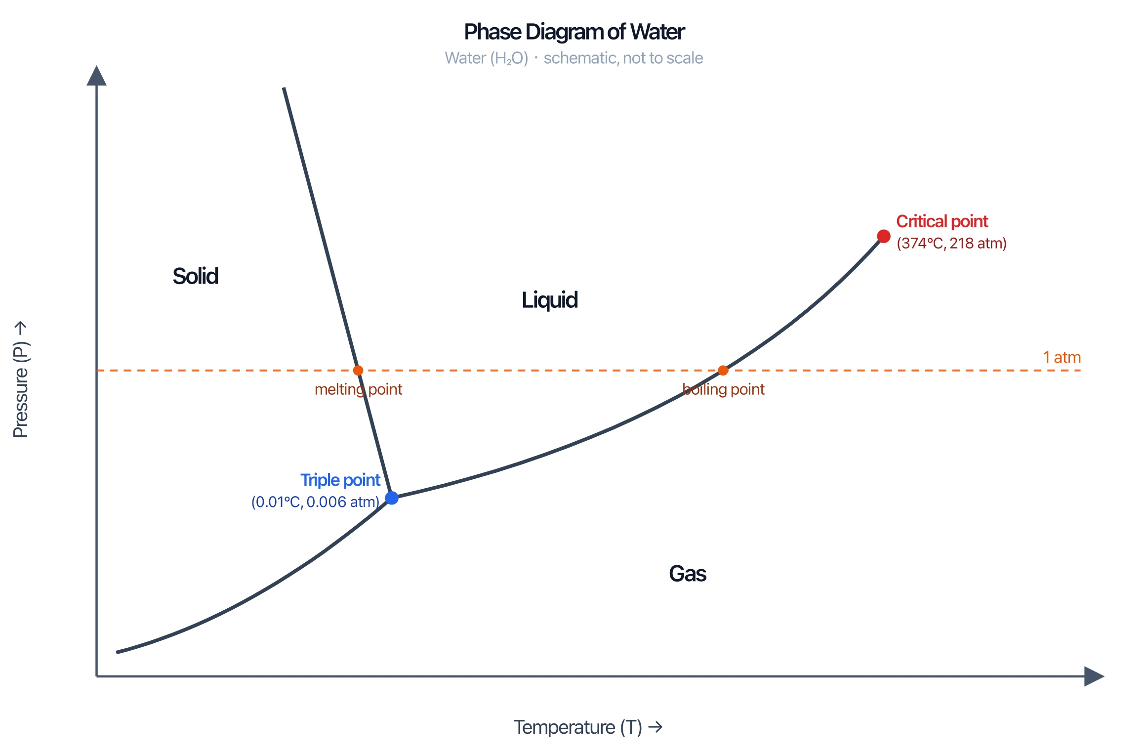
Phase Diagram Generator
Plot pressure-temperature phase diagrams for the same boiling and condensing behavior.
 Engineering
Schematic Diagram Maker
Lab and equipment schematics when the figure is an apparatus rather than a cycle.